1. The document discusses various concepts related to genotype by environment interaction (GxE) in plant breeding including stability analysis models. It introduces key terms like genotype, environment, phenotype, and patterns of GxE interaction.
2. Several stability analysis models are described including conventional models like ANOVA, regression models like Eberhart and Russell, and multiplicative models like AMMI and GGE biplot. Case studies demonstrate applications of models like AMMI biplots and GGE biplots.
3. The value of stability analysis is emphasized for identifying stable high-yielding genotypes, subdividing geographic regions, understanding actual genotypic performance, and deciding breeding strategies. Software tools can assist with stability analysis.
Stability parameters for comparing varieties (eberhart and russell 1966)Dhanuja Kumar
Phenotype is a result of genotype, environment and GE interaction. GENOTYPE- environment interactions are of major
importance to the plant breeder in developing
improved varieties. The performance of a single variety is not the same in all the environments. To identify a genotype whose performance is stable across environments various models were proposed. One such model was proposed by EBERHART and RUSSELL in 1966. Even after decades, this model is still preferred over others and used till date for stability analysis.
Stability analysis and G*E interactions in plantsRachana Bagudam
Gene–environment interaction is when two different genotypes respond to environmental variation in different ways. Stability refers to the performance with respective to environmental factors overtime within given location. Selection for stability is not possible until a biometrical model with suitable parameters is available to provide criteria necessary to rank varieties / breeds for stability. Different models of stability are discussed.
Advanced biometrical and quantitative genetics akshayAkshay Deshmukh
Additive and Multiplicative Model
Shifted Multiplicative Model
Analysis and Selection of Genotype
Methods and steps to select the best model
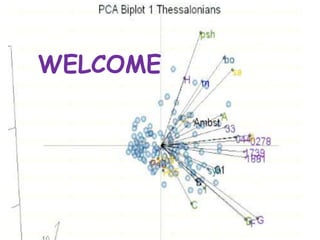
Bioplot and mapping genotype
Stability parameters for comparing varieties (eberhart and russell 1966)Dhanuja Kumar
Phenotype is a result of genotype, environment and GE interaction. GENOTYPE- environment interactions are of major
importance to the plant breeder in developing
improved varieties. The performance of a single variety is not the same in all the environments. To identify a genotype whose performance is stable across environments various models were proposed. One such model was proposed by EBERHART and RUSSELL in 1966. Even after decades, this model is still preferred over others and used till date for stability analysis.
Stability analysis and G*E interactions in plantsRachana Bagudam
Gene–environment interaction is when two different genotypes respond to environmental variation in different ways. Stability refers to the performance with respective to environmental factors overtime within given location. Selection for stability is not possible until a biometrical model with suitable parameters is available to provide criteria necessary to rank varieties / breeds for stability. Different models of stability are discussed.
Advanced biometrical and quantitative genetics akshayAkshay Deshmukh
Additive and Multiplicative Model
Shifted Multiplicative Model
Analysis and Selection of Genotype
Methods and steps to select the best model
Bioplot and mapping genotype
mechanisms creating heterosis in the genotypes at molecular level i.e., in the areas of transcriptomics, proteomics and metabolomics by DNA methylation, small RNAs, histone modifications and parent-of-origin effect
Heterotic group “is a group of related or unrelated genotypes from the same or different populations, which display similar combining ability and heterotic response when crossed with genotypes from other genetically distinct germplasm groups.”
Stability refers to the performance with respective changing environmental factors overtime within given location.
Selection for stability is not possible until a biometrical model with suitable parameters is available to provide criteria necessary to rank varieties / breeds for stability.
GGEBiplot analysis of genotype × environment interaction in Agropyron interme...Innspub Net
In order to identify genotypes of Agropyron intermedium with high forage yield and stability an experiment was carried out in the Research station of Kermanshah Iran.The 11 accessions were sown in a randomized complete block design with three replications under rainfed and irrigated conditions during 2013-21-014 cropping deasons. Combined analysis of variance indicated high significant differences for location, genotype and G × E interaction (GEI) at 1% level of probability. Mean comparisons over environments introduced G4, G3 and G5 with maximum forage yield over rainfed and irrigated conditions. Minimum forage yield was attributed to genotype G1. GGEbiplot analysis exhibited that the first two principal components (PCA) resulted from GEI and genotype effect justified 99.37% of total variance in the data set. The four environments under investigation fell into two apparent groups: irrigated and rainfed. The presence of close associations among irrigated (E1 and E3) and rainfed (E2 and E4) conditions suggests that the same information about the genotypes could be obtained from fewer test environments, and hence the potential to reduce testing cost.The which-won-where pattern of GGEbiplot introduced genotypes G3 and G4 as stable with high forage yield for rainfed condition, while G5 was stable with high yield for irrigated condition. According to the comparison of the genotypes with the Ideal genotype accessions G4, G3 and G9 were more favorable than all the other genotypes. Get more articles at: http://www.innspub.net/volume-6-number-4-april-2015-jbes/
QTL is a gene or the chromosomal region that affects a quantitative trait, which should be polymorphic (have allelic variation) to have an effect in a population, must be linked to a polymorphic marker allele to be detected. The QTL mapping consists of 4 steps, like the development of mapping population, generation of polymorphic marker data set among the parents, construction of linkage map, and finally the QTL analysis
All the above steps are described in these slides very briefly along with two case studies.
Introduction:
Proposed by Meuwissen et al. (2001)
GS is a specialized form of MAS, in which information from genotype data on marker alleles covering the entire genome forms the basis of selection.
The effects associated with all the marker loci, irrespective of whether the effects are significant or not, covering the entire genome are estimated.
The marker effect estimates are used to calculate the genomic estimated breeding values (GEBVs) of different individuals/lines, which form the basis of selection.
Why to go for genomic selection:
Marker-assisted selection (MAS) is well-suited for handling oligogenes and quantitative trait loci (QTLs) with large effects but not for minor QTLs.
MARS attempts to take into account small effect QTLs by combining trait phenotype data with marker genotype data into a combined selection index.
Based on markers showing significant association with the trait(s) and for this reason has been criticized as inefficient
The genomic selection (GS) scheme was to rectify the deficiency of MAS and MARS schemes. The GS scheme utilizes information from genome-wide marker data whether or not their associations with the concerned trait(s) are significant.
GEBV: Genomic Estimated Breeding Values-
The sum total of effects associated with all the marker alleles present in the individual and included in the GS model applied to the population under selection
Calculated on a single individual basis
Gene-assisted genomic selection:
A GS model that uses information about prior known QTLs, the targeted QTLs were accumulated in much higher frequencies than when the standard ridge regression was used
The sum total of effects associated with all the marker alleles present in the individual and included in the GS model applied to the population under selection
Calculated on a single individual basis
Population used:
Training population: used for training of the GS model and for obtaining estimates of the marker-associated effects needed for estimation of GEBVs of individuals/lines in the breeding population.
Breeding population: the population subjected to GS for achieving the desired improvement and isolation of superior lines for use as new varieties/parents of new improved hybrids.
Training population-
large enough: must be representative of the breeding population: max. trait variance with marker : by cluster analysis
should have either equal or comparable LD, LD decay rates with breeding populations
Updated by including individuals/lines from the breeding population
Training more than one generation
Low colinearity between markers is needed since high colinearity tends to reduce prediction accuracy of certain GS models. (colinearity disturbed by recombination)
Genomics, proteomics and metabolomics are the three core omics technologies, which respectively deal with the analysis of genome, proteome and metabolome of cells and tissues of an organism.
The shifted multiplicative model was developed by Cornelius and Seyedsadr in 1992.
SHMM is used to analyze the complete separability, genotypic separability, environmental separability, and inseparability of environment effects and genotypic effects.
Gregorius and Namkoong (1986) defined Separability as the property which is that cultivar effect is separable from environmental effect so that there is no rank.
The shifted multiplicative model (SHMM) is used in an exploratory step-down method for identifying subsets of environments in which genotypic effects are "separable" from environmental effects. Subsets of environments are chosen on the basis of a SHMM analysis of the entire data set. SHMM analyses of the subsets
may indicate a need for further subdivision and/or suggest that a different subdivision at the previous stage should be tried. The process continues until SHMM analysis indicates that a SHMM with only one multiplicative term and its "point of concurrence" outside (left or right) of the cluster of data points adequately fits the data in all subsets.
Genotype x Environment Interaction and Grain Yield Stability of Maize (Zea ma...Premier Publishers
Testing of genotypes in multi-environments is an important to estimate genotype x environment interaction (GEI) and identify stable genotypes with superior performance. The study was to evaluate different maize hybrids at multi-environments as well as to identify high yielding and stable maize hybrids. Twenty maize hybrids were tested across eight environments in a randomized complete block design in the 2015 cropping season. Combined analysis of variance and AMMI analysis showed that genotype, environment and GEI effect were highly significant (p < 0. 01) for grain yield. Genotype, environment and GEI explained 6.62, 84.87 and 4.50% of the total experimental variations, indicating the importance of environment for variations in grain yield. Mean grain yield of tested hybrids ranged from 4.98 t ha-1 in G2 to 7.51 t ha-1 in G16. As evident from significant GEI, performances of the hybrids were inconsistent across environments indicated that suitable to specific environment. Based on AMMI stability value and mean ranking of GGE biplot indicated that G18 (BH 546) had high grain yield (7.16 t ha-1) and more stable across tested environments. This study identified maize hybrids with high grain yield and stable across environments that need to be further validated for possible new maize variety release and or the newly released hybrid is used for possible commercial production.
Seventeen sesame genotypes were tested at ten environments in Tigray, Northern Ethiopia during 2014-2015 cropping seasons. Randomized Complete Block Designs (RCBD) with three replications was used in the study. According to the GGE bi-plot different sesame growing environments grouped into two mega-environments: The first mega-environment contained the favorable environments Dansha area with a vertex G4 and Sheraro area with winner G3 and the second environment included medium to low environments E2 (Humera-2), E4 (Dansha-2), E5 (Sheraro-1), E7 (Wargiba-1), E8 (Wargiba-2) and E9 (Maykadra) for seed yield. Three mega-environments identified for oil content: The 1st environment contained G12, G7 and G2 in the mega-environment group of Humera, Dansha and Gendawuha, The 2nd environment, Sheraro location contained G9 and the 3rd environment Wargiba, was containing G17. G1 (HuRC-4) identified as an “ideal” genotype and E1 (Humera-1) also identified as an ideal environment the most representative of the overall environments and the most powerful to discriminate genotypes. The multivariate approaches AMMI and GGEbi-plot were better for partitioning the GEI into the causes of variation. According to different stability models, G1, G7, and G3 were high yielder and the most stable both in terms of seed yield and oil content. Moreover, showed yield advantages over the released and local varieties. The stable genotypes recommended for wider areas while G14 and G4 were for specific favorable environments Sheraro and Dansha, respectively.
Grain Yield Stability in Three-way Cross Hybrid Maize Varieties using AMMI an...Premier Publishers
A study to evaluate three-way cross hybrid maize varieties for wide adaptability and stability was conducted in eight environments in Sierra Leone using AMMI and GGE biplot analysis. There were significant genotype and environment main effects, and genotype x environment interactions (GEI) effects. Differences due to environments accounted for 70.1% of the total treatments sum of squares while genotypes and genotype x environment interaction accounted for 9.9% and 20.0%, respectively. The first four interaction principal component axes (IPCA) were also highly significant and accounted for 38.7%, 25.2%, 14.3% and 8.6%, respectively of the total genotype x environment interaction variation. The polygon view of the GGE biplot revealed that hybrid G14 produced the highest grain yield in environments E1, E5 and E7 whereas G24 was adaptive in environments E6, E8, E3, E4 and E2. Hybrids G24, G9, G17 and G6 also produced high grain yields and were relatively stable. Both AMMI and GGE biplot effectively partitioned treatments sum of squares and were more appropriate in explaining genotype x environment interaction. The models also identified G24 as the most desirable hybrid in terms of high grain yield and stability across environments. Therefore, this hybrid is recommended for commercial release.
Nine groundnut varieties were tested across six environments in western Oromia, Ethiopia during 2013 main cropping season to evaluate the performance of groundnut varieties for kernel yield and their stability across environments. The varieties were arranged in randomized complete block design (RCBD) with three replications. Pooled analysis of variance for kernel yield showed significant (p≤0.01) differences among the varieties, environments and the genotype by environment interaction (GxE). Additive main effect and multiplicative interactions (AMMI) analysis showed highly significant (p≤0.01) differences for varieties, environments and their interaction on kernel yield. Similarly, the first and the second interaction principal component axis (IPCA1 and IPCA 2) were highly significant (p≤0.01) and explained 41.32 and 7.2% of the total GxE sum of squares, respectively. The environment, genotype and genotype by environment interaction accounted 14.7, 24.1 and 53.3% variations, respectively. This indicated the existence of considerable amounts of deferential response among the varieties to changes in growing environments and the deferential discriminating ability of the test environments. Shulamith and Bulki varieties showed the smallest genotype selection index (GSI) values and had the highest kernel yield and stability showing that these varieties had general adaptation in the tested environments. In the genotype and genotype by environment (GGE) biplot analysis, IPCA1 and IPCA 2 explained 63.5% and 22.4%, respectively, of genotype by environment interaction and made a total of 85.9%. GGE biplot analysis also confirmed Bulki and Shulamith varieties showed better stability and thus ideal varieties recommended for production in the test environments and similar agro-ecologies.
What is greenhouse gasses and how many gasses are there to affect the Earth.moosaasad1975
What are greenhouse gasses how they affect the earth and its environment what is the future of the environment and earth how the weather and the climate effects.
Earliest Galaxies in the JADES Origins Field: Luminosity Function and Cosmic ...Sérgio Sacani
We characterize the earliest galaxy population in the JADES Origins Field (JOF), the deepest
imaging field observed with JWST. We make use of the ancillary Hubble optical images (5 filters
spanning 0.4−0.9µm) and novel JWST images with 14 filters spanning 0.8−5µm, including 7 mediumband filters, and reaching total exposure times of up to 46 hours per filter. We combine all our data
at > 2.3µm to construct an ultradeep image, reaching as deep as ≈ 31.4 AB mag in the stack and
30.3-31.0 AB mag (5σ, r = 0.1” circular aperture) in individual filters. We measure photometric
redshifts and use robust selection criteria to identify a sample of eight galaxy candidates at redshifts
z = 11.5 − 15. These objects show compact half-light radii of R1/2 ∼ 50 − 200pc, stellar masses of
M⋆ ∼ 107−108M⊙, and star-formation rates of SFR ∼ 0.1−1 M⊙ yr−1
. Our search finds no candidates
at 15 < z < 20, placing upper limits at these redshifts. We develop a forward modeling approach to
infer the properties of the evolving luminosity function without binning in redshift or luminosity that
marginalizes over the photometric redshift uncertainty of our candidate galaxies and incorporates the
impact of non-detections. We find a z = 12 luminosity function in good agreement with prior results,
and that the luminosity function normalization and UV luminosity density decline by a factor of ∼ 2.5
from z = 12 to z = 14. We discuss the possible implications of our results in the context of theoretical
models for evolution of the dark matter halo mass function.
Slide 1: Title Slide
Extrachromosomal Inheritance
Slide 2: Introduction to Extrachromosomal Inheritance
Definition: Extrachromosomal inheritance refers to the transmission of genetic material that is not found within the nucleus.
Key Components: Involves genes located in mitochondria, chloroplasts, and plasmids.
Slide 3: Mitochondrial Inheritance
Mitochondria: Organelles responsible for energy production.
Mitochondrial DNA (mtDNA): Circular DNA molecule found in mitochondria.
Inheritance Pattern: Maternally inherited, meaning it is passed from mothers to all their offspring.
Diseases: Examples include Leber’s hereditary optic neuropathy (LHON) and mitochondrial myopathy.
Slide 4: Chloroplast Inheritance
Chloroplasts: Organelles responsible for photosynthesis in plants.
Chloroplast DNA (cpDNA): Circular DNA molecule found in chloroplasts.
Inheritance Pattern: Often maternally inherited in most plants, but can vary in some species.
Examples: Variegation in plants, where leaf color patterns are determined by chloroplast DNA.
Slide 5: Plasmid Inheritance
Plasmids: Small, circular DNA molecules found in bacteria and some eukaryotes.
Features: Can carry antibiotic resistance genes and can be transferred between cells through processes like conjugation.
Significance: Important in biotechnology for gene cloning and genetic engineering.
Slide 6: Mechanisms of Extrachromosomal Inheritance
Non-Mendelian Patterns: Do not follow Mendel’s laws of inheritance.
Cytoplasmic Segregation: During cell division, organelles like mitochondria and chloroplasts are randomly distributed to daughter cells.
Heteroplasmy: Presence of more than one type of organellar genome within a cell, leading to variation in expression.
Slide 7: Examples of Extrachromosomal Inheritance
Four O’clock Plant (Mirabilis jalapa): Shows variegated leaves due to different cpDNA in leaf cells.
Petite Mutants in Yeast: Result from mutations in mitochondrial DNA affecting respiration.
Slide 8: Importance of Extrachromosomal Inheritance
Evolution: Provides insight into the evolution of eukaryotic cells.
Medicine: Understanding mitochondrial inheritance helps in diagnosing and treating mitochondrial diseases.
Agriculture: Chloroplast inheritance can be used in plant breeding and genetic modification.
Slide 9: Recent Research and Advances
Gene Editing: Techniques like CRISPR-Cas9 are being used to edit mitochondrial and chloroplast DNA.
Therapies: Development of mitochondrial replacement therapy (MRT) for preventing mitochondrial diseases.
Slide 10: Conclusion
Summary: Extrachromosomal inheritance involves the transmission of genetic material outside the nucleus and plays a crucial role in genetics, medicine, and biotechnology.
Future Directions: Continued research and technological advancements hold promise for new treatments and applications.
Slide 11: Questions and Discussion
Invite Audience: Open the floor for any questions or further discussion on the topic.
Comparing Evolved Extractive Text Summary Scores of Bidirectional Encoder Rep...University of Maribor
Slides from:
11th International Conference on Electrical, Electronics and Computer Engineering (IcETRAN), Niš, 3-6 June 2024
Track: Artificial Intelligence
https://www.etran.rs/2024/en/home-english/
Richard's aventures in two entangled wonderlandsRichard Gill
Since the loophole-free Bell experiments of 2020 and the Nobel prizes in physics of 2022, critics of Bell's work have retreated to the fortress of super-determinism. Now, super-determinism is a derogatory word - it just means "determinism". Palmer, Hance and Hossenfelder argue that quantum mechanics and determinism are not incompatible, using a sophisticated mathematical construction based on a subtle thinning of allowed states and measurements in quantum mechanics, such that what is left appears to make Bell's argument fail, without altering the empirical predictions of quantum mechanics. I think however that it is a smoke screen, and the slogan "lost in math" comes to my mind. I will discuss some other recent disproofs of Bell's theorem using the language of causality based on causal graphs. Causal thinking is also central to law and justice. I will mention surprising connections to my work on serial killer nurse cases, in particular the Dutch case of Lucia de Berk and the current UK case of Lucy Letby.
THE IMPORTANCE OF MARTIAN ATMOSPHERE SAMPLE RETURN.Sérgio Sacani
The return of a sample of near-surface atmosphere from Mars would facilitate answers to several first-order science questions surrounding the formation and evolution of the planet. One of the important aspects of terrestrial planet formation in general is the role that primary atmospheres played in influencing the chemistry and structure of the planets and their antecedents. Studies of the martian atmosphere can be used to investigate the role of a primary atmosphere in its history. Atmosphere samples would also inform our understanding of the near-surface chemistry of the planet, and ultimately the prospects for life. High-precision isotopic analyses of constituent gases are needed to address these questions, requiring that the analyses are made on returned samples rather than in situ.
Cancer cell metabolism: special Reference to Lactate PathwayAADYARAJPANDEY1
Normal Cell Metabolism:
Cellular respiration describes the series of steps that cells use to break down sugar and other chemicals to get the energy we need to function.
Energy is stored in the bonds of glucose and when glucose is broken down, much of that energy is released.
Cell utilize energy in the form of ATP.
The first step of respiration is called glycolysis. In a series of steps, glycolysis breaks glucose into two smaller molecules - a chemical called pyruvate. A small amount of ATP is formed during this process.
Most healthy cells continue the breakdown in a second process, called the Kreb's cycle. The Kreb's cycle allows cells to “burn” the pyruvates made in glycolysis to get more ATP.
The last step in the breakdown of glucose is called oxidative phosphorylation (Ox-Phos).
It takes place in specialized cell structures called mitochondria. This process produces a large amount of ATP. Importantly, cells need oxygen to complete oxidative phosphorylation.
If a cell completes only glycolysis, only 2 molecules of ATP are made per glucose. However, if the cell completes the entire respiration process (glycolysis - Kreb's - oxidative phosphorylation), about 36 molecules of ATP are created, giving it much more energy to use.
IN CANCER CELL:
Unlike healthy cells that "burn" the entire molecule of sugar to capture a large amount of energy as ATP, cancer cells are wasteful.
Cancer cells only partially break down sugar molecules. They overuse the first step of respiration, glycolysis. They frequently do not complete the second step, oxidative phosphorylation.
This results in only 2 molecules of ATP per each glucose molecule instead of the 36 or so ATPs healthy cells gain. As a result, cancer cells need to use a lot more sugar molecules to get enough energy to survive.
introduction to WARBERG PHENOMENA:
WARBURG EFFECT Usually, cancer cells are highly glycolytic (glucose addiction) and take up more glucose than do normal cells from outside.
Otto Heinrich Warburg (; 8 October 1883 – 1 August 1970) In 1931 was awarded the Nobel Prize in Physiology for his "discovery of the nature and mode of action of the respiratory enzyme.
WARNBURG EFFECT : cancer cells under aerobic (well-oxygenated) conditions to metabolize glucose to lactate (aerobic glycolysis) is known as the Warburg effect. Warburg made the observation that tumor slices consume glucose and secrete lactate at a higher rate than normal tissues.
(May 29th, 2024) Advancements in Intravital Microscopy- Insights for Preclini...Scintica Instrumentation
Intravital microscopy (IVM) is a powerful tool utilized to study cellular behavior over time and space in vivo. Much of our understanding of cell biology has been accomplished using various in vitro and ex vivo methods; however, these studies do not necessarily reflect the natural dynamics of biological processes. Unlike traditional cell culture or fixed tissue imaging, IVM allows for the ultra-fast high-resolution imaging of cellular processes over time and space and were studied in its natural environment. Real-time visualization of biological processes in the context of an intact organism helps maintain physiological relevance and provide insights into the progression of disease, response to treatments or developmental processes.
In this webinar we give an overview of advanced applications of the IVM system in preclinical research. IVIM technology is a provider of all-in-one intravital microscopy systems and solutions optimized for in vivo imaging of live animal models at sub-micron resolution. The system’s unique features and user-friendly software enables researchers to probe fast dynamic biological processes such as immune cell tracking, cell-cell interaction as well as vascularization and tumor metastasis with exceptional detail. This webinar will also give an overview of IVM being utilized in drug development, offering a view into the intricate interaction between drugs/nanoparticles and tissues in vivo and allows for the evaluation of therapeutic intervention in a variety of tissues and organs. This interdisciplinary collaboration continues to drive the advancements of novel therapeutic strategies.
Deep Behavioral Phenotyping in Systems Neuroscience for Functional Atlasing a...Ana Luísa Pinho
Functional Magnetic Resonance Imaging (fMRI) provides means to characterize brain activations in response to behavior. However, cognitive neuroscience has been limited to group-level effects referring to the performance of specific tasks. To obtain the functional profile of elementary cognitive mechanisms, the combination of brain responses to many tasks is required. Yet, to date, both structural atlases and parcellation-based activations do not fully account for cognitive function and still present several limitations. Further, they do not adapt overall to individual characteristics. In this talk, I will give an account of deep-behavioral phenotyping strategies, namely data-driven methods in large task-fMRI datasets, to optimize functional brain-data collection and improve inference of effects-of-interest related to mental processes. Key to this approach is the employment of fast multi-functional paradigms rich on features that can be well parametrized and, consequently, facilitate the creation of psycho-physiological constructs to be modelled with imaging data. Particular emphasis will be given to music stimuli when studying high-order cognitive mechanisms, due to their ecological nature and quality to enable complex behavior compounded by discrete entities. I will also discuss how deep-behavioral phenotyping and individualized models applied to neuroimaging data can better account for the subject-specific organization of domain-general cognitive systems in the human brain. Finally, the accumulation of functional brain signatures brings the possibility to clarify relationships among tasks and create a univocal link between brain systems and mental functions through: (1) the development of ontologies proposing an organization of cognitive processes; and (2) brain-network taxonomies describing functional specialization. To this end, tools to improve commensurability in cognitive science are necessary, such as public repositories, ontology-based platforms and automated meta-analysis tools. I will thus discuss some brain-atlasing resources currently under development, and their applicability in cognitive as well as clinical neuroscience.
Multi-source connectivity as the driver of solar wind variability in the heli...Sérgio Sacani
The ambient solar wind that flls the heliosphere originates from multiple
sources in the solar corona and is highly structured. It is often described
as high-speed, relatively homogeneous, plasma streams from coronal
holes and slow-speed, highly variable, streams whose source regions are
under debate. A key goal of ESA/NASA’s Solar Orbiter mission is to identify
solar wind sources and understand what drives the complexity seen in the
heliosphere. By combining magnetic feld modelling and spectroscopic
techniques with high-resolution observations and measurements, we show
that the solar wind variability detected in situ by Solar Orbiter in March
2022 is driven by spatio-temporal changes in the magnetic connectivity to
multiple sources in the solar atmosphere. The magnetic feld footpoints
connected to the spacecraft moved from the boundaries of a coronal hole
to one active region (12961) and then across to another region (12957). This
is refected in the in situ measurements, which show the transition from fast
to highly Alfvénic then to slow solar wind that is disrupted by the arrival of
a coronal mass ejection. Our results describe solar wind variability at 0.5 au
but are applicable to near-Earth observatories.
Professional air quality monitoring systems provide immediate, on-site data for analysis, compliance, and decision-making.
Monitor common gases, weather parameters, particulates.
Introduction:
RNA interference (RNAi) or Post-Transcriptional Gene Silencing (PTGS) is an important biological process for modulating eukaryotic gene expression.
It is highly conserved process of posttranscriptional gene silencing by which double stranded RNA (dsRNA) causes sequence-specific degradation of mRNA sequences.
dsRNA-induced gene silencing (RNAi) is reported in a wide range of eukaryotes ranging from worms, insects, mammals and plants.
This process mediates resistance to both endogenous parasitic and exogenous pathogenic nucleic acids, and regulates the expression of protein-coding genes.
What are small ncRNAs?
micro RNA (miRNA)
short interfering RNA (siRNA)
Properties of small non-coding RNA:
Involved in silencing mRNA transcripts.
Called “small” because they are usually only about 21-24 nucleotides long.
Synthesized by first cutting up longer precursor sequences (like the 61nt one that Lee discovered).
Silence an mRNA by base pairing with some sequence on the mRNA.
Discovery of siRNA?
The first small RNA:
In 1993 Rosalind Lee (Victor Ambros lab) was studying a non- coding gene in C. elegans, lin-4, that was involved in silencing of another gene, lin-14, at the appropriate time in the
development of the worm C. elegans.
Two small transcripts of lin-4 (22nt and 61nt) were found to be complementary to a sequence in the 3' UTR of lin-14.
Because lin-4 encoded no protein, she deduced that it must be these transcripts that are causing the silencing by RNA-RNA interactions.
Types of RNAi ( non coding RNA)
MiRNA
Length (23-25 nt)
Trans acting
Binds with target MRNA in mismatch
Translation inhibition
Si RNA
Length 21 nt.
Cis acting
Bind with target Mrna in perfect complementary sequence
Piwi-RNA
Length ; 25 to 36 nt.
Expressed in Germ Cells
Regulates trnasposomes activity
MECHANISM OF RNAI:
First the double-stranded RNA teams up with a protein complex named Dicer, which cuts the long RNA into short pieces.
Then another protein complex called RISC (RNA-induced silencing complex) discards one of the two RNA strands.
The RISC-docked, single-stranded RNA then pairs with the homologous mRNA and destroys it.
THE RISC COMPLEX:
RISC is large(>500kD) RNA multi- protein Binding complex which triggers MRNA degradation in response to MRNA
Unwinding of double stranded Si RNA by ATP independent Helicase
Active component of RISC is Ago proteins( ENDONUCLEASE) which cleave target MRNA.
DICER: endonuclease (RNase Family III)
Argonaute: Central Component of the RNA-Induced Silencing Complex (RISC)
One strand of the dsRNA produced by Dicer is retained in the RISC complex in association with Argonaute
ARGONAUTE PROTEIN :
1.PAZ(PIWI/Argonaute/ Zwille)- Recognition of target MRNA
2.PIWI (p-element induced wimpy Testis)- breaks Phosphodiester bond of mRNA.)RNAse H activity.
MiRNA:
The Double-stranded RNAs are naturally produced in eukaryotic cells during development, and they have a key role in regulating gene expression .
2. 2
Ashwini Gopal Lamani
PALM6001
Sr. M.Sc.(Agri.)
Department of Genetics and
Plant Breeding
SEMINAR - I
UNIVERSITY OF AGRICULTURAL SCIENCES, BANGALORE
COLLEGE OF AGRICULTURE, V C FARM, MANDYA
‘Development of Concept of Stability
Analysis in Plant Breeding’
5. What is GXE interaction??
‘The differential response of genotypes from one
environment to another is known as Genotype by
Environment interaction’
5
Kang and Gorman, (1989)
6. Patterns of the genotype behavior in different environments outlining
the two fundamental types of interaction, considering only a simple
case of two genotypes and two environments.
Ferreira et al., (2006) 6
8. Significance of Genotype and
Environment Interaction
Identify differences in environmental variation.
Subdivision of geographic region into relatively
homogeneous sub-regions
Actual genotypic performance
Deciding breeding strategies
8
9. Phenotypic stability
Well buffered variety.
Two concepts: a. Biological concept
b. Agronomic concept
Population buffering: heterogeneous
population.
Individual buffering: pure line varieties or
single crosses.
Allard and Bradshaw (1964)
10. Detection of G×E interaction
10
MLT- with replicated trials, several
locations, several years
Test for homogeneity of experimental
error by Bartlett’s test
Pooled analysis
Find genotype and G×E significance
from pooled ANOVA
Stability analysis using statistical
models
12. 1. Conventional Model
12
A in E1 A in E2
Yield
1. Stability Factor Model-Lewis (1954)
S.F= XHE
XLE
SF=1, Stable
genotype
13. Conti.. 1. Conventional Model
2. Basic ANOVA model
13Elias et al., (2016)
Where,
𝛾𝑖𝑗𝑘 =yield response variable
µ=overall mean
αi= genotypic effect
βj= jth environmental effect
(αβ)ij= interaction effect
εijk= residual error
14. ANOVA for g genotypes evaluated at e
environments in trials having r replications
14
Source of
variance
df SS MSS F value
Genotypes
(G)
g -1 GSS GMS
Environment
s(E)
e - 1 EnSS EnMS
Replication
within
environments
e(r -1) RSS RMS
G x E (g-1) (e -1) GESS GEMS
Error e (g -1)(r-1) ESS EMS
15. Basic ANOVA model
Advantages
i. Quantifies magnitude of
classifiable main effects and
interactions
ii. Presence of G×E
iii. Identifying environments as
TPE when
no significant G×E is
present and
similarity in the
magnitude of G×E
Disadvantages
i. Does not describe the
pattern of G and E
response
ii. Requires replications
within environments.
iii. Quantifies G×E in single
dimension
iv. Assumes homogeneity of
experimental errors.
Elias et al., (2016)
17. 2. Regression Models
1. Finley and Wilkinson model (1963)
2. Eberhart and Russel model (1966)
3. Perkins and Jinks model (1968)
4. Freeman and Perkins model (1971)
17
18. 1. Finley and Wilkinson model (1963)
Genotypic mean (gi).
Regression coefficient (bi) as phenotypic
stability.
18
19. 19
A generalized interpretation of genotypic pattern obtained when, genotypic
regression co-efficients are plotted against genotypic mean
20. 2. Eberhart and Russel model (1966)
Three parameters of stability:
(i) Genotype mean (gi).
(ii) Regression value bi (predictable linear response)
(iii) Deviation from linearity (unpredictable non
linear response)
20
sdi
2
21. 2. Eberhart and Russel model (1966)
General features
MSS due to G and
GXE interaction is
partitioned into
three components
E(linear)
GXE(linear)
Pooled deviation
Stable with:
High mean yield(X)
bi=1
approaching
zero
21
22. Format of ANOVA (Eberhart and Russel Model,1966)
SV df SS MSS
Genotypes (v-1)
Env.+GE v(n-1)
Env.(linear) 1
GE(linear) v-1
Pooled deviations v(n-1)
G1 n-2
G2 n-2
.
Gv n-2
Pooled error n(r-1)(v-1)
Total nv-1 22
23. Perkins and Jinks model (1968)
• Three stability parameters viz.,
– mean (Yi ),
– regression coefficient (bi) and
– deviation from regression ( sdi )
• Regression of G x E interaction on
environmental index was obtained rather than
regression on mean performance.
23
2
24. Freeman and Perkins model (1971)
• Joint regression analysis
• Three stability parameters viz.,
– mean (Yi),
– regression coefficient (bi)
– mean square deviation from regression [S2di]
• Environment is completely independent.
24
25. Advantages of Regression Models.
• Response pattern over environment and stability of
genotype.
• Environment quality in single dimension.
.
• GEI signal retained as much as possible.
25Malosetti et al., (2013)
26. Disadvantages of Regression Models.
Fails to explain large portion of G×E
Assumes linear relationship between G×E and
environment means
Model does not fit if extreme environments are
involved.
Less informative where G×E is too complex
Assumes homogeneity of environment errors
Environment characters is based on single
dimension
26
Malosetti et al., (2013)
28. Multiplicative Models
Explains complex G×E
Assumes fixed effect
Eliminates much of noise in data.
Explains pattern of GxE interactions.
28Elias et al., (2016)
32. AMMI Model
Additive Main Effect and Multiplicative
Interaction.
Partitions variations into:
Additive effect (G,E)by ANOVA
Multiplicative effect(GXE) by PCA
Use biplots
32Gauch, H. G., (2013)
33. AMMI model
33
Yge= yield of the genotype (g) in the environment (e);
μ= grand mean
αg= genotype mean deviation
βe= environment mean deviation;
N = No. of IPCAs (Interaction Principal Component Axis)
retained in the model
λn= singular value for IPCA axis n
ϒgn= genotype eigenvector values for IPCA axis n
δen= environment eigenvector values for IPCA axis n
ρge= the residual.
Zobel et al., (1998)
35. 35
Illustration of a biplot graph with PC1 vs mean yield, presenting the
main types of genotypes and patterns of stability and adaptation.
Ferreira et al., (2006)
36. 36
Zobel et al., (1998)
Biplot of the AMMI model for a New York soybean yield trial with 7 genotypes
grown in 35 environments. Genotype and environment codes are given in materials
and methods. The grand mean is represented by a ‘’ plus ‘’
37. 37
Biplot from the AMMI model used to describe GEI in the maize example data. Gray
circles represent genotypes, and filled triangles environments , with triangles pointing
in the direction of increasing GEI (at origin GEI = 0). The projection of two genotypes
(G041andG091)on the NS92a axis is shown by a dashed line.
Malosetti et al., (2013)
38. Evaluation of Genotype × Environment
Interaction in Rice
Based on AMMI Model in Iran
38
Sharifi et al., 2017
39. 39
AMMI 1 biplot for nine rice genotypes and nine rice environment
46. Comparing Two Statistical Models for Studying
Genotype x Environment Interaction and Stability
Analysis in Flax
46Mohsen, A. A. and Amein, M. M. (2016)
47. Table1. The environments used in this study
Code Growing
season
N
rate(k
g/fed)
Description
E1 2011-12 20 E1 is 1st Fertilizer rate(20kgN per fed) in the first
season
E2 2011-12 35 E2 is 2nd fertilizer rate(35kg/fed) in the first season
E3 2011-12 50 E3 is the 3rd fertilizer rate (50kg/fed) in the first
season
E4 2012-13 20 E4 is the 4th fertilizer rate(20kg/fed) in the second
season
E5 2012-13 35 E5 is the 5th fertilizer rate( 35 kg/fed) in the second
season
E6 2012-13 50 E6 is the 1st fertilizer rate (50kg/fed) in the second
season
47
Mohsen and Amein (2016)
48. 48
Estimates of stability and adaptability parameters of straw yield
(ton/fed) for 7 flax cultivars across 6 environments.
Mohsen and Amein (2016)
50. 50
Table 6. The estimates of stability and adaptability parameters of seed
yield(ton/fed) for 7 flax cultivars across 6 environments.
Mohsen and Amein (2016)
51. 51
Fig 2. The relationship between the regression coefficients and seed
yield(ton/fed) for 7 flax cultivars. The horizontal solid line represents the mean
coefficient of regression and the vertical solid line denotes the mean seed yield.
53. 53
Fig. 5. Ranking of cultivars based on mean and stability GGE biplot of for 7
cultivars under six environments.
54. Shifted Multiplicative Model
• Developed by Seyedsadr and Cornelius(1992)
• Main effects not fitted into ANOVA.
• PCA is performed on the combined effects
rather than just interaction.
54
Elias et al., (2016)
55. Shifted Multiplicative Model
• Shift parameter ϴ, to minimize the residual
error
• Used to identify environment in which
genotypic effects are separable from
environmental effects
55
Elias et al., (2016)
56. Genotype Regression Model(GREG)
• Each genotype as multiple regression on the
interaction.
• Main effects from the G effect, multiplicative
term for E+GE.
56
Elias et al., (2016)
58. Use of external variables in Models
1. Factorial Regression Model:
Estimate genotypic sensitivity to environmental
covariates.
Not effective for multi-colinearity of large external
variable.
2. Partial Least Square Model:
no limit to number of external variables used
58
Elias et al., (2016)
59. Use of Mixed Effects in Models
Random effects
Effective for unbalanced data
No restriction for replications within
environment
Considers heterogeneous variance
Eg: BLUPs, FAMM, BLUEs
59
Elias et al., (2016)
60. To know QTL×E
1. Single environment analysis.
2. Genomic best linear unbiased
prediction(GBLUP) model.
3. GBLUP model with deviation
coefficient for each environment
assumed.
4. M×E GBLUP
60
Elias et al., (2016)
61. Non-parametric methods
Based on ranks of genotypes across
environment.
No assumptions
Easy for interpretation
Stable genotype: having same rank across
environments.
Eg: Shukla(1972), Nassar and Huhn(1987),
Kang(1988), Fox et al.,1990, Thennarasu(1995)
61Elias et al., (2016)
62. Softwares used in stability analysis
Windostat
Genstat
Genes software
MATLAB
SAS program
R program
62