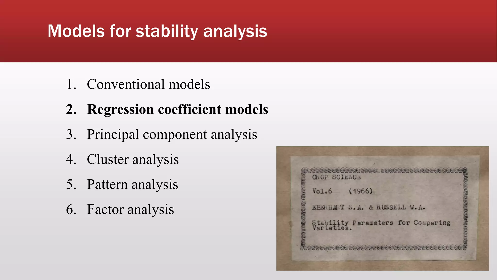
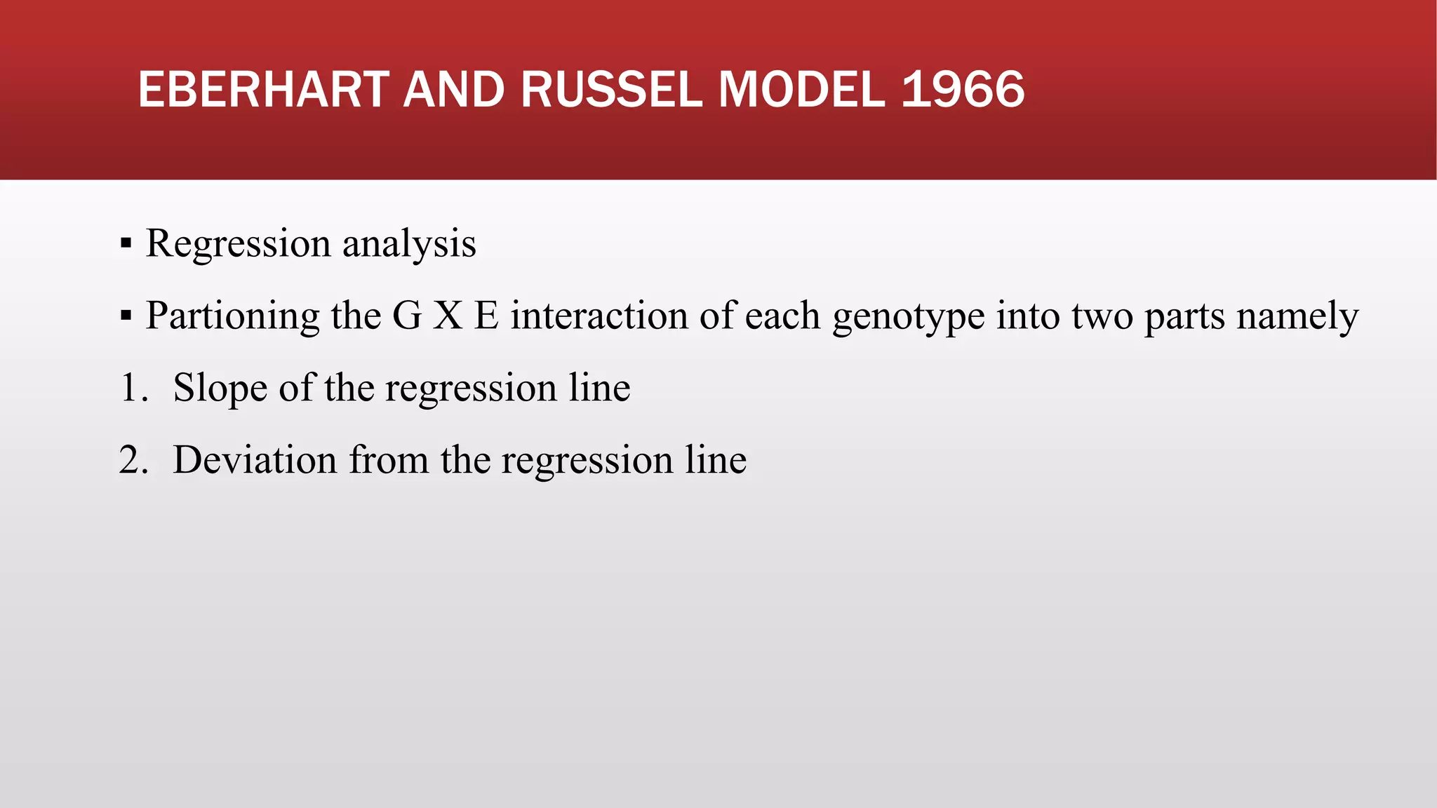
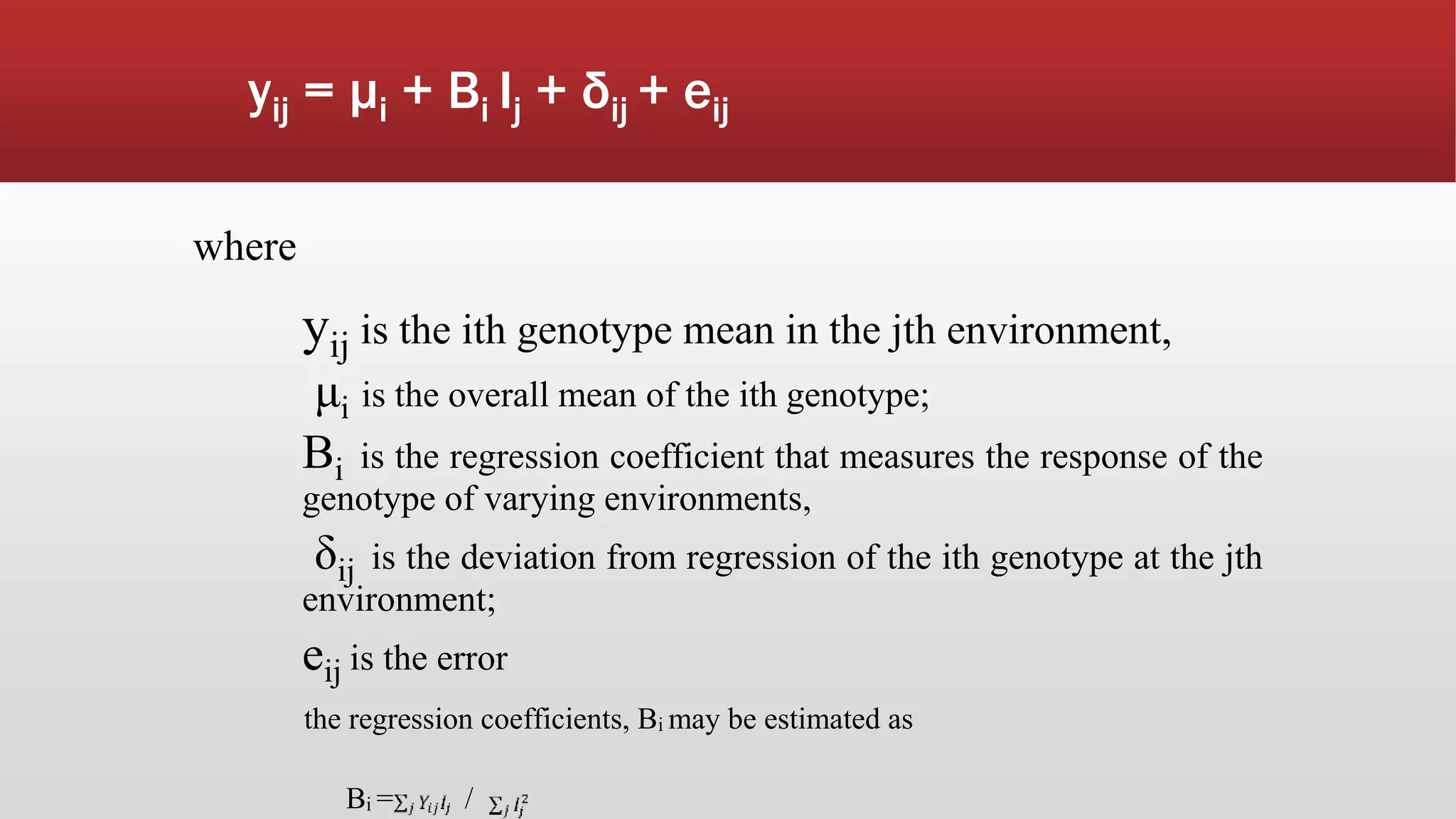
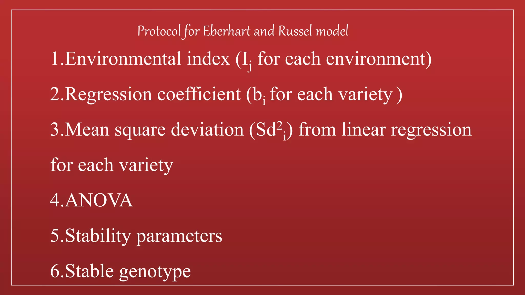
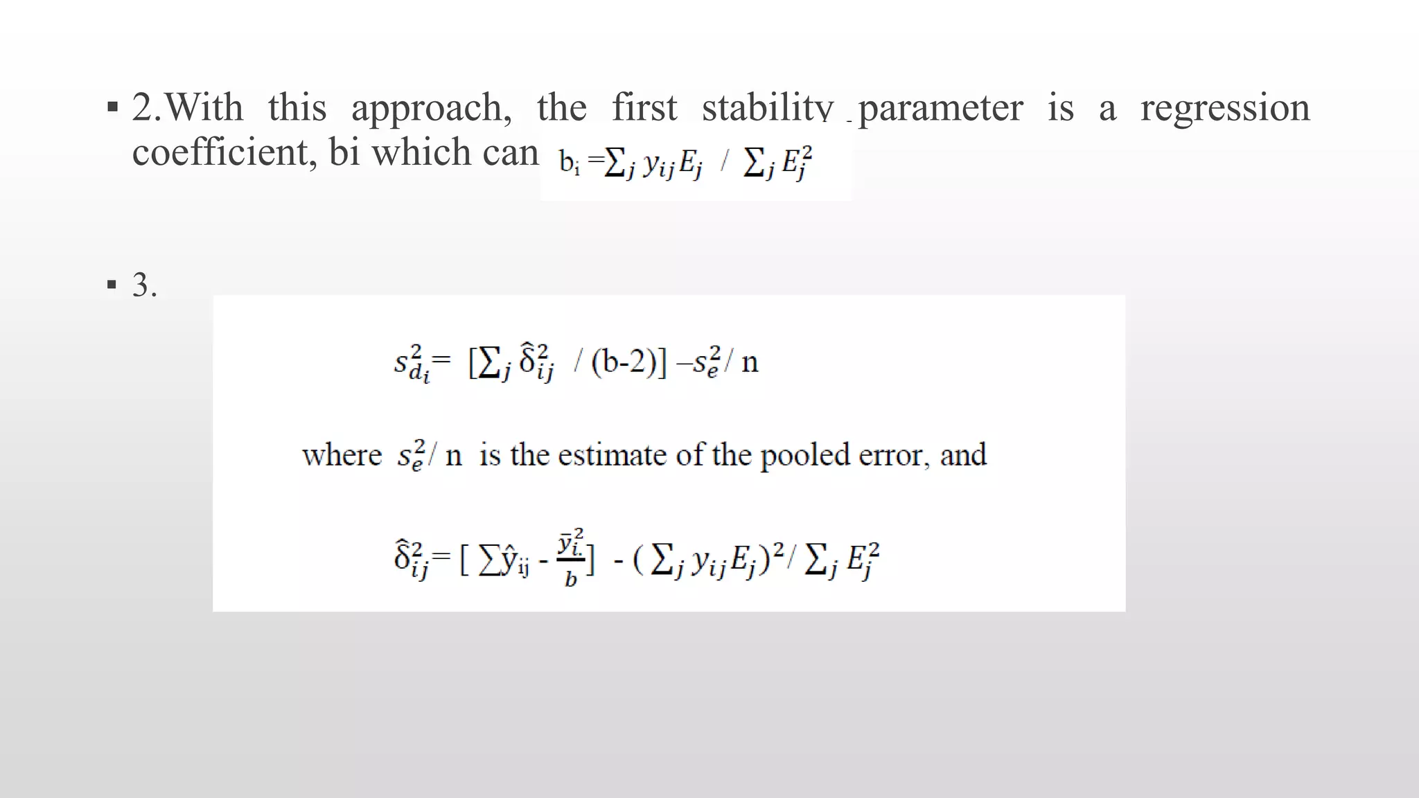
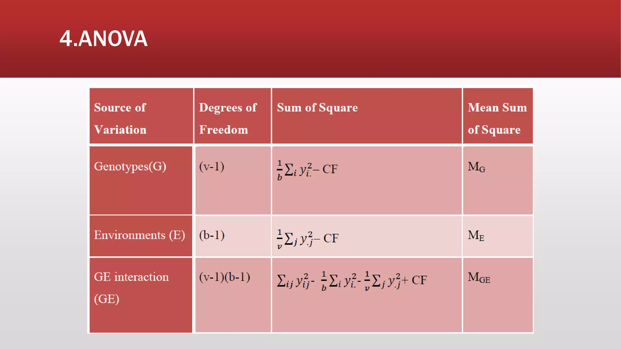
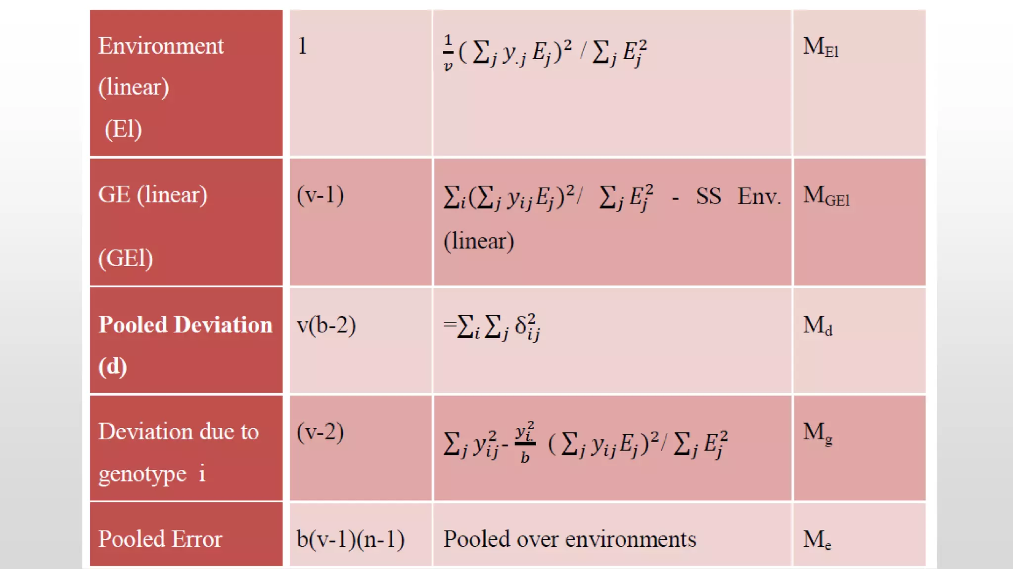
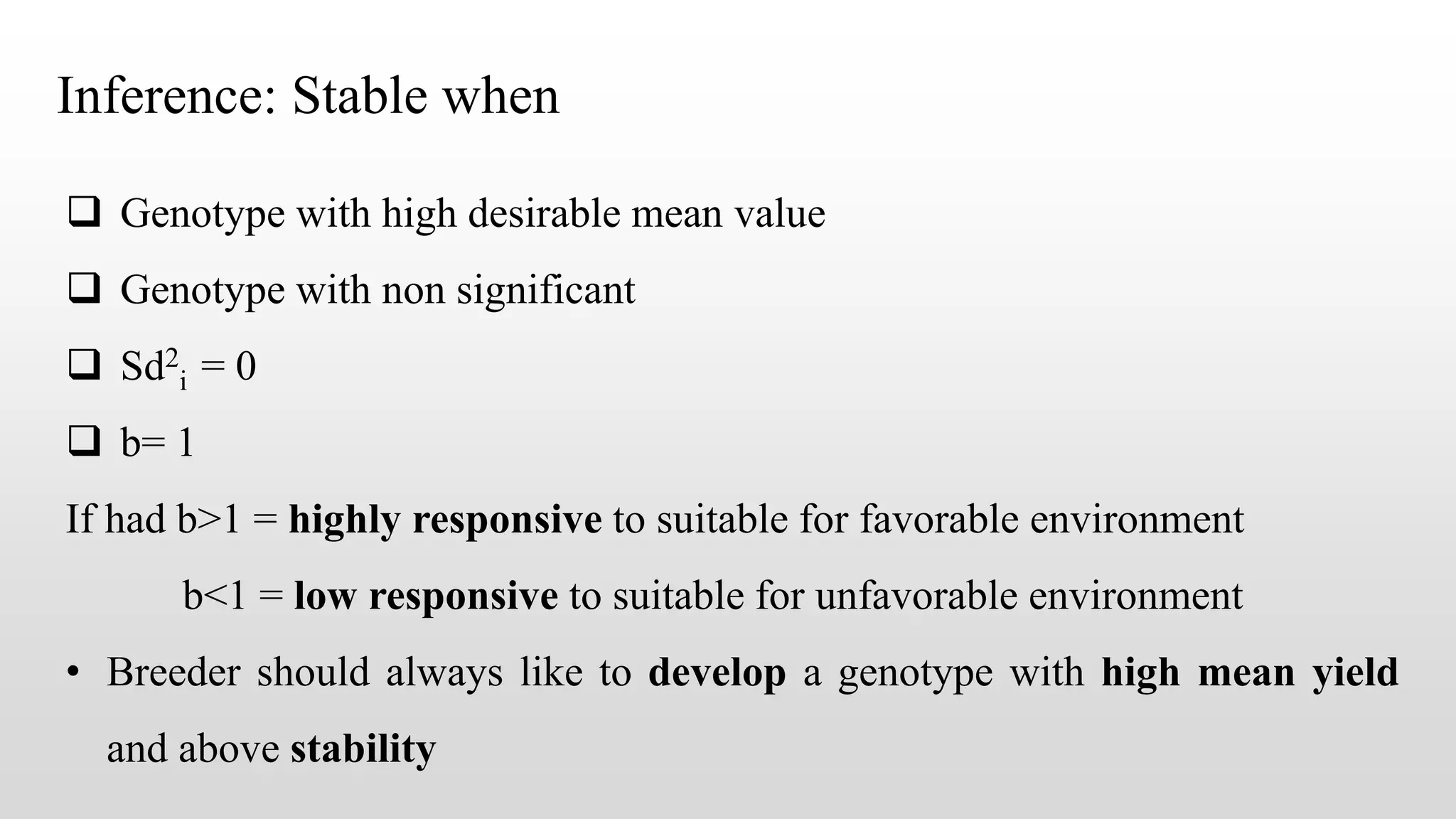
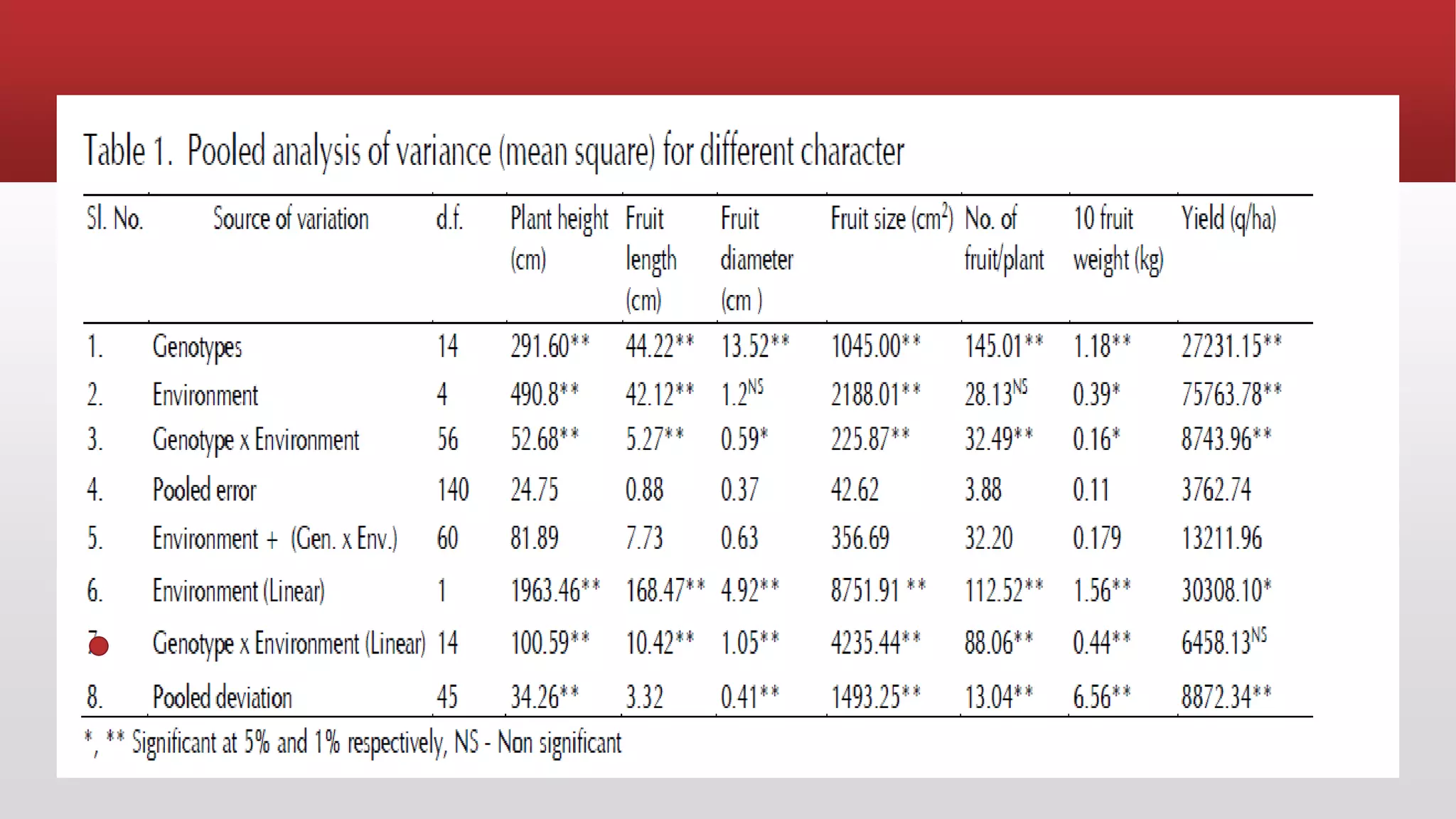
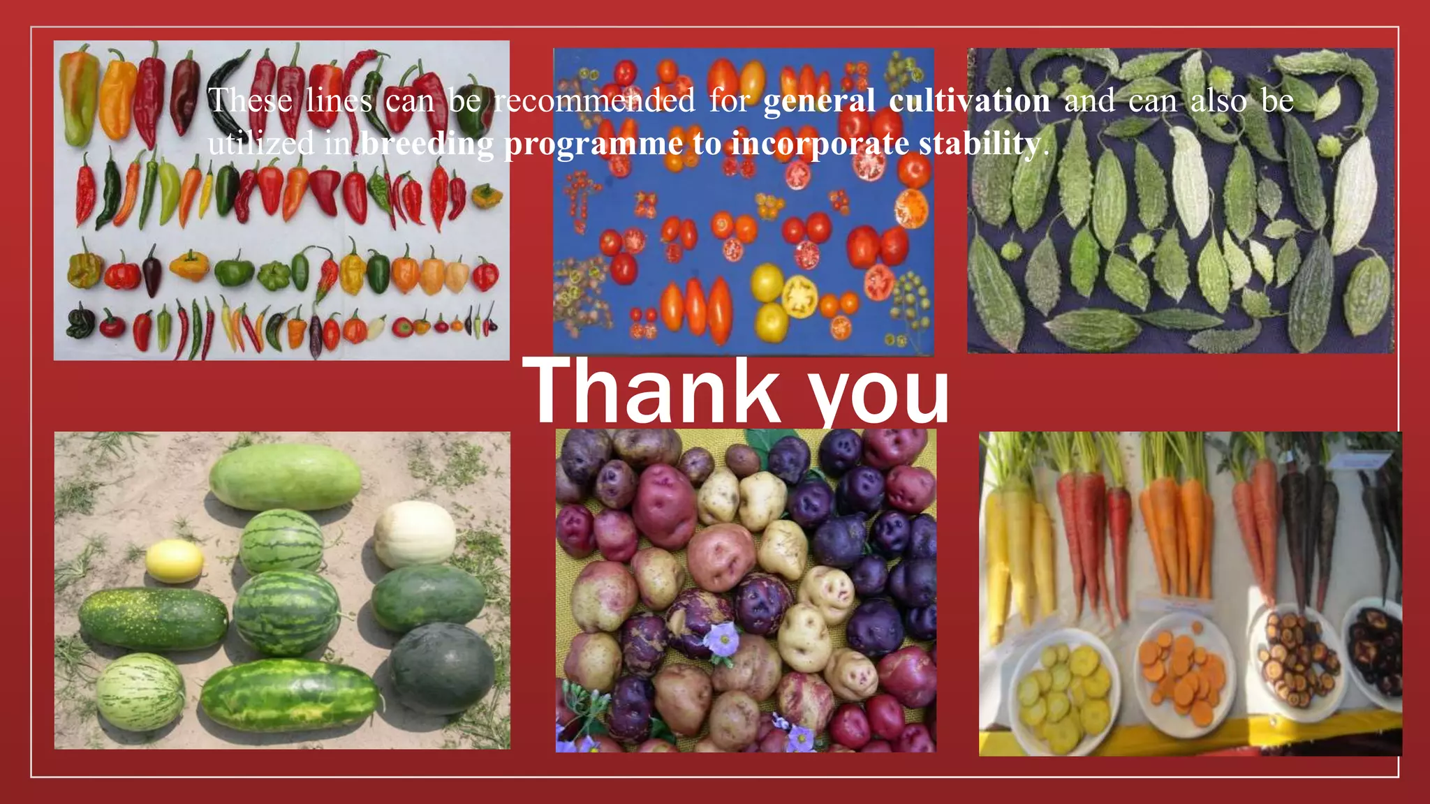
STABILITY ANALYSIS
EBERHART AND RUSSEL MODEL
(1966)
Dealt with G X E
Submitted by
S.ADHIYAMAAN (2017603401)
I-M.Sc.,VEGETABLE SCIENCE
DEPT. OF VEGETABLE CROPS
HC & RI, TNAU, CBE.- 641 003
DEFINITON
▪ P = G+E
▪ P is not same to change in environment
▪ Interplay in the effect of genetic and non-genetic on development is
termed as genotype-environment interaction
- (Comstock and Moll,1963)
▪ So G X E = major thing for breeder to evolve a new variety
ENVIRONMENT
▪ Micro environment
▪ Macro environment
▪ Allard and Bradshaw 1964 coined two terms
▪ Predictable environmental variations
▪ Unpredictable environmental variations
Climate resilient plant varieties
G X E INTERACTION
▪ Develop genotypes that can withstand unpredictable transient
environmental fluctuations.
▪ Phenotypic stability concepts
▪ Biological concept
▪ Agronomical concept
STABILITY AND BUFFERING (SIMMONDS 1962 )
▪ Specific genotypic adaptation
▪ General genotypic adaptation
▪ Specific population adaptation
▪ General population adaptation
▪ Consistently superior performance over several environments - Frey 1964
▪ Genetic homeostasis
▪ Physiological homeostasis
▪ Stability in performance 1) Population buffering 2) Individual buffering
Wider adaptable variety
Radish - Pusa Himani
Cabbage - Pusa Sambandh
Cucumber- Pusa Uday
Bottle gourd – Pusa Santushi
Models for stability analysis
1. Conventional models
2. Regression coefficient models
3. Principal component analysis
4. Cluster analysis
5. Pattern analysis
6. Factor analysis
EBERHART AND RUSSEL MODEL 1966
▪ Regression analysis
▪ Partioning the G X E interaction of each genotype into two parts namely
1. Slope of the regression line
2. Deviation from the regression line
yij = μi + Bi Ij + δij + eij
where
yij is the ith genotype mean in the jth environment,
μi is the overall mean of the ith genotype;
Bi is the regression coefficient that measures the response of the
genotype of varying environments,
δij is the deviation from regression of the ith genotype at the jth
environment;
eij is the error
the regression coefficients, Bi may be estimated as
Bi = /
1.Environmental index (Ij for each environment)
2.Regression coefficient (bi for each variety )
3.Mean square deviation (Sd2
i) from linear regression
for each variety
4.ANOVA
5.Stability parameters
6.Stable genotype
Protocol for Eberhart and Russel model
▪ 2.With this approach, the first stability parameter is a regression
coefficient, bi which can be estimated by
▪ 3.
4.ANOVA
The model provides a means of partitioning the GE interaction of each
genotype into two parts:
(i) the variation due to the response of genotype to varying environmental
indices (sums of square due to regression), and
(ii) the deviation from regression on the environmental indices.
# Hence, the second stability parameter (Sd2
i) played a very important
role as the estimated variance
Inference: Stable when
 Genotype with high desirable mean value
 Genotype with non significant
 Sd2
i = 0
 b= 1
If had b>1 = highly responsive to suitable for favorable environment
b<1 = low responsive to suitable for unfavorable environment
• Breeder should always like to develop a genotype with high mean yield
and above stability
STABILITY ANALYSIS FOR GROWTH AND YIELD ATTRIBUTES
IN BRINJAL
Author : S.N.S. Chaurasia, Major Singh and Mathura Rai
Journal : Vegetable Science
Indian Institute of Vegetable Research, Varanasi-221 305
(U.P.)
Materials and Methods
▪ Genotypes :15
▪ Three replications
▪ These lines were evaluated for five years in randomized block design
▪ Plot size : 3.6 x 3.0 m
▪ Spacing : 60 x 60 cm
▪ August month in all the five years
Observations recorded :
▪ plant height, fruit length, fruit diameter, fruit size, number of fruits/plants
Thank you
These lines can be recommended for general cultivation and can also be
utilized in breeding programme to incorporate stability.

Stability analysis

  • 1.
    STABILITY ANALYSIS EBERHART ANDRUSSEL MODEL (1966) Dealt with G X E Submitted by S.ADHIYAMAAN (2017603401) I-M.Sc.,VEGETABLE SCIENCE DEPT. OF VEGETABLE CROPS HC & RI, TNAU, CBE.- 641 003
  • 2.
    DEFINITON ▪ P =G+E ▪ P is not same to change in environment ▪ Interplay in the effect of genetic and non-genetic on development is termed as genotype-environment interaction - (Comstock and Moll,1963) ▪ So G X E = major thing for breeder to evolve a new variety
  • 3.
    ENVIRONMENT ▪ Micro environment ▪Macro environment ▪ Allard and Bradshaw 1964 coined two terms ▪ Predictable environmental variations ▪ Unpredictable environmental variations Climate resilient plant varieties
  • 4.
    G X EINTERACTION ▪ Develop genotypes that can withstand unpredictable transient environmental fluctuations. ▪ Phenotypic stability concepts ▪ Biological concept ▪ Agronomical concept
  • 5.
    STABILITY AND BUFFERING(SIMMONDS 1962 ) ▪ Specific genotypic adaptation ▪ General genotypic adaptation ▪ Specific population adaptation ▪ General population adaptation ▪ Consistently superior performance over several environments - Frey 1964 ▪ Genetic homeostasis ▪ Physiological homeostasis ▪ Stability in performance 1) Population buffering 2) Individual buffering
  • 6.
    Wider adaptable variety Radish- Pusa Himani Cabbage - Pusa Sambandh Cucumber- Pusa Uday Bottle gourd – Pusa Santushi
  • 7.
    Models for stabilityanalysis 1. Conventional models 2. Regression coefficient models 3. Principal component analysis 4. Cluster analysis 5. Pattern analysis 6. Factor analysis
  • 8.
    EBERHART AND RUSSELMODEL 1966 ▪ Regression analysis ▪ Partioning the G X E interaction of each genotype into two parts namely 1. Slope of the regression line 2. Deviation from the regression line
  • 9.
    yij = μi+ Bi Ij + δij + eij where yij is the ith genotype mean in the jth environment, μi is the overall mean of the ith genotype; Bi is the regression coefficient that measures the response of the genotype of varying environments, δij is the deviation from regression of the ith genotype at the jth environment; eij is the error the regression coefficients, Bi may be estimated as Bi = /
  • 10.
    1.Environmental index (Ijfor each environment) 2.Regression coefficient (bi for each variety ) 3.Mean square deviation (Sd2 i) from linear regression for each variety 4.ANOVA 5.Stability parameters 6.Stable genotype Protocol for Eberhart and Russel model
  • 11.
    ▪ 2.With thisapproach, the first stability parameter is a regression coefficient, bi which can be estimated by ▪ 3.
  • 12.
  • 14.
    The model providesa means of partitioning the GE interaction of each genotype into two parts: (i) the variation due to the response of genotype to varying environmental indices (sums of square due to regression), and (ii) the deviation from regression on the environmental indices. # Hence, the second stability parameter (Sd2 i) played a very important role as the estimated variance
  • 15.
    Inference: Stable when Genotype with high desirable mean value  Genotype with non significant  Sd2 i = 0  b= 1 If had b>1 = highly responsive to suitable for favorable environment b<1 = low responsive to suitable for unfavorable environment • Breeder should always like to develop a genotype with high mean yield and above stability
  • 16.
    STABILITY ANALYSIS FORGROWTH AND YIELD ATTRIBUTES IN BRINJAL Author : S.N.S. Chaurasia, Major Singh and Mathura Rai Journal : Vegetable Science Indian Institute of Vegetable Research, Varanasi-221 305 (U.P.)
  • 17.
    Materials and Methods ▪Genotypes :15 ▪ Three replications ▪ These lines were evaluated for five years in randomized block design ▪ Plot size : 3.6 x 3.0 m ▪ Spacing : 60 x 60 cm ▪ August month in all the five years Observations recorded : ▪ plant height, fruit length, fruit diameter, fruit size, number of fruits/plants
  • 21.
    Thank you These linescan be recommended for general cultivation and can also be utilized in breeding programme to incorporate stability.