The document discusses the genotype x environment (GxE) interaction and its influence on the phenotype of rice genotypes across varying environmental conditions. It elaborates on different models for analysis, including the AMMI model, which combines ANOVA and principal components analysis to evaluate genotypic performances and environmental impacts. The study aims to identify high-yielding and stable rice hybrids suitable for diverse environments, utilizing various statistical methods for analysis.

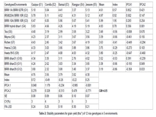
1. Submitted to
DR.K.B.ESWARI,
Associate
professor,
Dept of GPBR

2. The interaction between the genotype
and environment that produces the
phenotype is called as Genotype x
Environmental Interaction.
P = G + E + GE
Genotypes respond differently across
a range of environments i.e., the
relative performance of varieties
depends on the environment.

3. Environmental variable can be divided into 2
groups (Allard and Bradshaw , 1964)
1.Predictable environment factor
2.Unpredictable factor
Predictable factors include permanent features
of environment which are under human control
such as soil type,planting date, row spacing,
rows of new trend application.
Unpredictable factors are those which
fluctuate inconsistently like rainfall,
temperature, relative humidity not under
control are called unpredictable environment
conditions.

4. The environment refers to the external
conditions that affect expression of
genes of an individual genotype.
Environment can be classified into two
groups ( Comstock and Moll , 1963)
a) macro environment
b) micro environment

5. Refers to the environment with variables having
large and easily recognisable effect.
Main features:
1.The environment affects are easily
detectable such as fertilizer doses, planting
dates, spacing, irrigation schedules.
2.Macro environment is controlled by
Predictable factors such as soil type, planting
dates and close spacing.
3. It is under human control

6. The environment of a single organism
/genotype as opposed to that of another
growing at the same time in almost the same
place is referred to as micro environment.
Main features:
1.The environment effects are not easily
recognizable such as differences in humidity
, temperature, etc.. at the same place.
2.Micro environment is governed by
unpredictable factors like rain fall,
temperature, relative humidity which
fluctuate inconsistently.
3.It is not under human control.

7. It refers to those changes in structure or
function of an individual/population which lead to
better survival in a given environment is known
as adaptation.
Main features:
₭ Adaptation favours those characters which are
advantageous for survival and through which an
individual acquires adaptive value or fitness.
₭ In the process of adaptation survival is the
main concern.
₭ Natural selection plays an important role in the
process of adaptation.
ADAPTATION

8. 
TYPES OF ADAPTATION
There are four types of adaptation
1.Specific genotypic adaptation
2.General genotypic adaptation
3.Specific population adaptation
4.General population adaptation
Factors affecting adaptability:
 Heterogeneity.
Heterozygosity.
Genetic polymorphism.
Mode of pollination.

9. Stability refers to the performance with
respective changing environmental
factors overtime within given location.
selection for stability is not possible until
a biometrical model with suitable
parameters is available to provide criteria
necessary to rank varieties / breeds for
stability.
Low magnitude of G.E interaction involves
the consistent performance of a population
over variable environments.

10. It consists of following steps:
Location / environment wise analysis of
variance.
pooled analysis of variance for all the
locations/ environments.
If G.E interaction is found significant
,stability analysis can be carried out using
one of the four methods:
1.Finlay and Wilkinson model (1963)
2.Eberhat and Russell model(1966)
3.Perkins and Jinks model(1968)
4.Freeman and Perkins model (1971)

11. Used two parameters
1)Mean performance over environments.
2)Regression performance in different
environments.
The following inferences can be drawn:
1)The regression coefficient of unity indicates
average stability
2)If the regression coefficient is >1,it means
below average stability
3)If the regression coefficient is <1,it means
above average stability.
4)Regression coefficient of 0 would
express absolute stability.

12. MERITS
Analysis of this model is simple.
2 parameters- mean yield over locations and
regression coefficient are used to asses
the phenotypic stability.
DEMERITS
The deviations from the regression line are not
estimated which are important for the
stability analysis.
Greater emphasis is given on mean performance
over environments than regression
coefficients.

13. It is the most popular and useful model.
In 1966 both made further improvement in stability
analysis by partitioning the G.E interaction of
each
variety into 2 parts. one is slope of the regression line ,
second is deviation from regression line.
In this model total variance is first divided into 2
components:
-genotypes
-environment plus interaction (E+G*E)
The second component is further divided in
to 3 components.
I. Environment linear
II. G.E linear
III. Pooled deviations
Sum of squares due to pooled deviations are further
divided into sum of squares due to individual genotype.

14. This model consists of three parameters
a)mean yield over locations
b)regression coefficient =bi
C)Deviation from regression =s²di
Analysis of stability parameters is simple as
compared to other models of stability
analysis.
The degree of freedom for environment is
1.
It requires less area hence less expensive when
compared to other models.
It does not provide independent estimation for

15. Source of variation Degrees of freedom
Genotypes g-1
E+ G*E interaction g(e-1)
environment (linear) 1
G.E linear g-1
pooled deviations g(e-2)
genotype-1 e-2
genotype-2
Pooled error
e-2
ge(r-1)

16. Merits:
It measures three parameters of stability
A=mean yield over environments
B=regression coefficient
C=deviation from regression
line
 It provides more reliable information on stability than
Finlay and Wilkinson model.
Analysis is simple.
Demerits:
 estimation of mean performance and environment index is
not independent.
 There is a combined estimation of sum of squares of
environment and interactions which is not proper.
Eberhart and Russell (1956) defined stable variety as
one with a regression coefficient of unity(b=1) and a
minimum deviation from the regression

17. In this model total variance is first divided into 3
components.
1)genotypes
2)environments
3)genotypes x environment
G-E variance is sub
divided into
a) heterogeneity due to
regression
b) sum of square due
to remainder
This model is less
expensive than Freeman
and Perkins.
It requires less area
for experimentation.

18. Source of variation Degrees of freedom
Genotypes g-1
Environment e-1
Genotype x environment (g-1)(e-1)
Heterogeneity among regressions g-1
Remainder (g-1)(e-2)
Error ge(r-1)

19. In this model total variance is first divided into 3
components.
1)Genotypes 2)environment 3) G*E
The environmental s.s is sub divided into 2
components
a) combined regression b) residual 1
The interaction variance is also subdivided into two
parts
a)homogeneity of regression b) residual 2
This model also includes 3 parameters like Eberhart
and Russell model and provides independent
estimation of mean performance and environmental
index.
The degree of freedom for environment is e-2 like
perkins and jinks model.
Analysis of this model is more difficult and

20. Source of variation Degrees of freedom
Genotypes g-1
Environment e-1
Combined
regression
1
residual (1) e-2
Interaction(GxE) (g-1)(e-2)
Heterogeneity of
regressions
g-1
residual (2)
error
(g-1)(e-2)
ge(r-1)

21. AMMI is a combination of ANOVA for the main
effects of the genotypes and the environment
together with principal components analysis of
the genotype-environment interaction.
Method for analyzing GEI to identify patterns of
interaction and reduce background noise.
May provide more reliable estimates of genotype
performance than the mean across sites.
Biplots help to visualize relationships among
genotypes and environments; show both main and
interaction effects.

22. Yijl =  + Gi + Ej + (kikjk)
+ eijl
Where,
•Yij is the observed mean yield of the ith genotype in jth
environment
•μ is the general mean
•Gi and Ej represent the effects of the genotype
and environment
•λk is the singular value of the kth axis in the PCA
•αik is the eigenvector of the ith genotype for the
kth axis
•γjk is the eigenvector of the jth environment for the kth
axis
•n is the number of principal components in the model
AMMI Model

23. source df SS MS F
TOTAL (ger- 1)
Treatment (ge -1)
Genotype (g -1)
Environment (e-1)
Interaction
IPCA
1
IPCA
2
Residual
(g-1) (e-1)
blocks (r-1)
error (r-1) (ge -1)
Analysis of variance for stability – AMMI
Model

24. PRINCIPAL COMPONENTS
usually the first principal component (CP1)
represents responsesof the genotypes
that are proportional to the
environments, which are associated with
the GxE interaction without change of the
range.
The second principal component (CP2)
provides information about cultivation
locations that are not proportional to the
environments, indicating that those are
responsible of the GxE crossover
interaction.

25. Biplot allows the observation in the same
graph of the genotypes (points) and the
environments (vectors), and (2) the exploration
of patterns attributable to the effects of
GxE interaction.
In the biplot, the angles between the vectors
that represent genotypes and environments show
the interaction, and the distances from the
origin indicate the degree of interaction that
the genotypes show throughout the
environments or vice versa.
Graphical representation of numerical results
often allows a straight forward
interpretation of GEI.
BIPLOT
S

27. General interpretation
◦ genotypes that occur close to particular
environments on the IPCA2 vs IPCA1
biplot show specific adaptation to those
environments
◦ a genotype that falls near the center of
the biplot (small IPCA1 and IPCA2
values) may have broader adaptation

28. How many IPCAs (interaction principal component
axes) are needed to adequately explain patterns
in the data?
◦ Rule of thumb - discard higher order
IPCAs until total SS due to discarded IPCA's
~ SSE.
◦ Usually need only the first 2 PC axes to
adequately explain the data (IPCA1 and
IPCA2). This model is referred to as AMMI2.
Approach is most useful when G x location
effects are more important than G x
year effects

29. Name of the journal – Journal of
radiation research
Year of publishing – 2014
Authors of the research paper -Anowara
Akter1*, Jamil Hassan M1, Umma Kulsum M1, Islam
MR1, Kamal Hossain1 and Mamunur Rahman M2*
1Plant Breeding Division, Bangladesh Rice Research
Institute, Bangladesh
2Senior Scientific Officer, Farm Management
Division, Bangladesh

30. Genotype x environment interaction and stability
performance were investigated on grain yield
with 12 rice genotypes in five environments.
The ANOVA for grain yield revealed highly
significant (P<0.01) for genotypes, environments
and their interactions.
The significant interaction indicated that
the genotypes respond differently across the
different environments.

31. The AMMI model is a hybrid model involving both
additive and multiplicative components of two
way data structure which enabled a breeder to
get precise prediction on genotypic potentiality
and environmental influences on it.
AMMI uses ordinary ANOVA to analyze the main
effects (additive part) and PCA to analyze the
non additive residual left over by the ANOVA .
The main objectives of the present study are
to identify more high yielding stable promising
hybrids and to determine the areas where rice
hybrids would be adapted by AMMI model.

32. The experiments were conducted at five districts
namely Gazipur(E1), Comilla (E2), Barisal (E3),
Rangpur (E4) and Jessore (E5) representing five
different agro-ecological zones (AEZ) of
Bangladesh.
Twelve genotypes consisting of 3 advanced lines
(BRRI 1A/ BRRI 827R(G1), IR58025A/ BRRI
10R (G2) and BRRI 10A/ BRRI 10R (G3)),
6released hybrids (BRRI hybrid
dhan1(G4), Tea (G5), Mayna (G6),Richer (G7),
Heera-2 (G8) and Heeta 99-5 (G9)), and 3
inbred check varieties (BRRI
dhan31 (G10), BRRI dhan33 (G11) and BRRI
dhan39(G12)) were used as experimental

33. The experiments were carried out in a randomized
complete block design (RCBD), with 3
replications.
21 days old seedlings were transplanted in 20
square meter plot using single seedling per hill at
a spacing of 20 cm×15cm.
Fertilizers were applied @ 150:100:70:60:10
kg/ha Urea, TSP,MP, gypsum and ZnSO4,
respectively.
Standard agronomic practices were followed and
plant protection measures were taken as required.
The grain yield data for 12 genotypes in 5
environments were subjected to AMMI analysis
of variance using statistical analysis package
software Cropstat version 6.1

34. ANOVA

36. Figure 1: AMMI 1 Biplot for grain yield (tha-1) of 12
rice genotypes (G) and five environments (E)using
genotypic and environmental scores.

37. Figure 2: AMMI 2 Biplot for grain yield (tha-1) showing the interaction of
IPCA2 against IPCA1 scores of 12 rice genotypes (G) in five
environments (E).

38. The mean grain yield value of genotypes averaged
over environments indicated that G3 had the
highest (5.99tha-1) and G12 the lowest yield
(3.19 tha-1), respectively.
It is noted that the variety G3 showed higher
grain yield than all other varieties over all
the environments.
The genotypes (G1), (G2), (G3) and (G4) were
hardly affected by the G x E interaction and thus
would perform well across a wide range of
environments.

39. Name of the journal;-Advances in Biological
Research
Year of publishing;-2009
Authors of the research paper;-A. Anandan, R.
Eswaran, T. Sabesan and M. Prakash.
Department of Agricultural Botany, Faculty of
Agriculture, Annamalai University, T.N.

40. ABSTRACT:
The objective of the present investigation was
to analyse the pattern of Genotype x
Environment (G x E) interaction for grain yield
of 46 genotypes by Additive Main effects
and Multiplicative Interaction (AMMI) model
using the data generated from three saline
stress environments of east coastal region of
Tamil Nadu, India.
The results showed highly significant genotypic
and G x E interaction.
The G x E interaction influenced the relative
ranking of the genotypes across saline
stress environment condition.

41. The developed cultivars should adapt to a
wide range of target environments, is the
eventual goal of plant breeders. Hence,
pattern of response of genotypes is
studied by testing genotypes in different
environments to study G X E interaction.
AMMI offers on appropriate first statistical
analysis of yield trials that may have a G x
E interaction . The objectives of this study
were to assess the extent of G x E
interaction and to select the stable
genotypes of rice

42. 46 rice genotypes from different parts of India
were evaluated at Plant Breeding Research Farm,
Faculty of Agriculture, Annamalai University,
Annamalai,East coastal region
of Tamil Nadu, India.
With soil pH of 8 to 8.5 and EC of 2.51 to 2.8 dSm .
The each genotype was evaluated in three seasons viz.,
E1 (Kharif, 2006), E2 (Kharif, 2007) and E3
(Rabi, 2007).
For all trials, the design used was RCBD with
three replications.
The plot had 10sq.m with spacing of 20 cm
between environments and rows and 20 cm between
plants.
Management practices were uniformly adapted to
all seasons as per the recommendation for rice

44. source df SS MS F
Treatments 137 905.60 6.61 216.78**
0.02 0.77
Genotypes 45
Environments 2
Interactions 90
IPCA 1
46
Residuals 44
Error
270
865.30 19.23 630.56**
36.50 18.24 5.43**
3.90 0.04 1.42*
2.90 0.06 2.04**
1.00
8.20 0.03

45. G
2
6

46. The genotypes which had IPCA score
nearest to zero are G24, G26, G27, G32
G34, G35, G39 and G45.
Among the above mentioned stable
genotypes, G45, G26, G27 G35 and G34
exhibited above average grain yield
and indicated that these genotypes
were well adaptable to saline
environment condition

47. SUBMITTED BY
B.RACHANA
RAM/16-45
DEPARTMENT OF
GENETICS AND
PLANT BREEDING