The document summarizes the solution to calculating the average leftover length of dental floss after cutting segments from two rolls until one runs out. It uses a binomial distribution to calculate the probability that the process ends with a given leftover length on one roll. Approximating the binomial coefficient using a Gaussian function allows simplifying the expression for the average leftover length to (2/√π)√Ld, where L is the initial total floss length and d is the segment length. So the average leftover amount is proportional to the geometric mean of the total length and segment length.

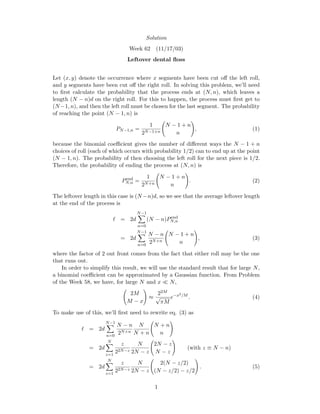
1. Solution
Week 62 (11/17/03)
Leftover dental floss
Let (x, y) denote the occurrence where x segments have been cut off the left roll,
and y segments have been cut off the right roll. In solving this problem, we’ll need
to first calculate the probability that the process ends at (N, n), which leaves a
length (N − n)d on the right roll. For this to happen, the process must first get to
(N −1, n), and then the left roll must be chosen for the last segment. The probability
of reaching the point (N − 1, n) is
PN−1,n =
1
2N−1+n
N − 1 + n
n
, (1)
because the binomial coefficient gives the number of different ways the N − 1 + n
choices of roll (each of which occurs with probability 1/2) can to end up at the point
(N − 1, n). The probability of then choosing the left roll for the next piece is 1/2.
Therefore, the probability of ending the process at (N, n) is
Pend
N,n =
1
2N+n
N − 1 + n
n
. (2)
The leftover length in this case is (N −n)d, so we see that the average leftover length
at the end of the process is
= 2d
N−1
n=0
(N − n)Pend
N,n
= 2d
N−1
n=0
N − n
2N+n
N − 1 + n
n
, (3)
where the factor of 2 out front comes from the fact that either roll may be the one
that runs out.
In order to simplify this result, we will use the standard result that for large N,
a binomial coefficient can be approximated by a Gaussian function. From Problem
of the Week 58, we have, for large N and x N,
2M
M − x
≈
22M
√
πM
e−x2/M
. (4)
To make use of this, we’ll first need to rewrite eq. (3) as
= 2d
N−1
n=0
N − n
2N+n
N
N + n
N + n
n
= 2d
N
z=1
z
22N−z
N
2N − z
2N − z
N − z
(with z ≡ N − n)
= 2d
N
z=1
z
22N−z
N
2N − z
2(N − z/2)
(N − z/2) − z/2
. (5)
1

2. Using eq. (4) to rewrite the binomial coefficient gives (with M ≡ N − z/2, and
x ≡ z/2)
≈ 2d
N
z=1
Nz
2N − z
e−z2/4(N−z/2)
π(N − z/2)
≈
d
√
πN
N
z=0
ze−z2/(4N)
≈
d
√
πN
∞
0
ze−z2/(4N)
dz
= 2d
N
π
. (6)
In obtaining the second line above, we have kept only the terms of leading order
in N. The exponential factor guarantees that only z values up to order
√
N will
contribute. Hence, z is negligible when added to N.
Without doing all the calculations, it’s a good bet that the answer should go like√
N d, but it takes some effort to show that the exact coefficient is 2/
√
π.
In terms of the initial length of floss, L ≡ Nd, the average leftover amount can
be written as ≈ (2/
√
π)
√
Ld. So we see that is proportional to the geometric
mean of L and d.
2