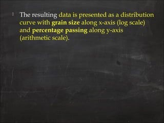
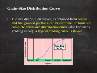
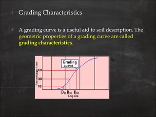
Downloaded 687 times


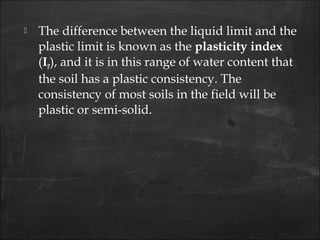
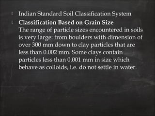
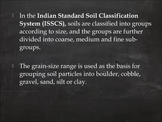
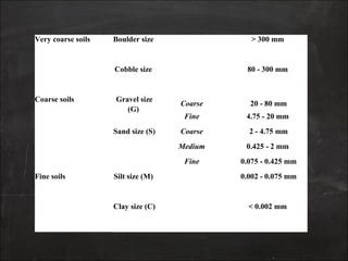
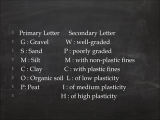
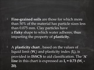
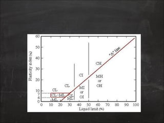
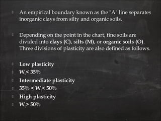
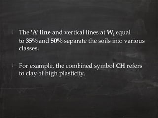
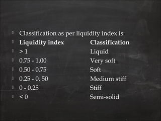
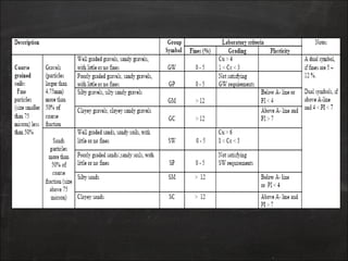
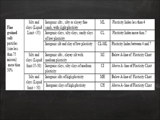

This document discusses soil classification systems. It provides information on classifying soils based on their grain size, plasticity properties, and engineering behavior. The key points are: - Soils are classified into groups like gravel, sand, silt, and clay based on particle size using systems like the Indian Standard Classification System. Additional criteria describe grading. - The plasticity of fine-grained soils is assessed using limits like liquid limit and plastic limit to classify them as low, intermediate, or high plasticity. - Classification helps describe and group soils based on meaningful engineering properties that influence permeability, compressibility, and shear strength for foundation and construction purposes.


