This document summarizes Arthur Charpentier's presentation on econometrics and statistical learning techniques. It discusses different perspectives on modeling data, including the causal story, conditional distribution story, and explanatory data story. It also covers topics like high dimensional data, computational econometrics, generalized linear models, goodness of fit, stepwise procedures, and testing in high dimensions. The presentation provides an overview of various statistical and econometric modeling techniques.

1. Arthur Charpentier
Econometrics: Learning from ‘Statistical Learning’ Techniques
Arthur Charpentier (Université de Rennes 1 & UQàM)
Chaire ACTINFO
Covéa, Paris, June 2016
http://freakonometrics.hypotheses.org
@freakonometrics 1

2. Arthur Charpentier
Econometrics: Learning from ‘Statistical Learning’ Techniques
Arthur Charpentier (Université de Rennes 1 & UQàM)
Professor, Economics Department, Univ. Rennes 1
In charge of Data Science for Actuaries program, IA
Research Chair actinfo (Institut Louis Bachelier)
(previously Actuarial Sciences at UQàM & ENSAE Paristech
actuary in Hong Kong, IT & Stats FFSA)
PhD in Statistics (KU Leuven), Fellow Institute of Actuaries
MSc in Financial Mathematics (Paris Dauphine) & ENSAE
Editor of the freakonometrics.hypotheses.org’s blog
Editor of Computational Actuarial Science, CRC
@freakonometrics 2

3. Arthur Charpentier
Agenda
“the numbers have no way of speaking for them-
selves. We speak for them. [· · · ] Before we de-
mand more of our data, we need to demand more
of ourselves ” from Silver (2012).
- (big) data
- econometrics & probabilistic modeling
- algorithmics & statistical learning
- different perspectives on classification
- boostrapping, PCA & variable section
see Berk (2008), Hastie, Tibshirani & Friedman
(2009), but also Breiman (2001)
@freakonometrics 3

4. Arthur Charpentier
Data and Models
From {(yi, xi)}, there are different stories behind, see Freedman (2005)
• the causal story : xj,i is usually considered as independent of the other
covariates xk,i. For all possible x, that value is mapped to m(x) and a noise
is attached, ε. The goal is to recover m(·), and the residuals are just the
difference between the response value and m(x).
• the conditional distribution story : for a linear model, we usually say
that Y given X = x is a N(m(x), σ2
) distribution. m(x) is then the
conditional mean. Here m(·) is assumed to really exist, but no causal
assumption is made, only a conditional one.
• the explanatory data story : there is no model, just data. We simply
want to summarize information contained in x’s to get an accurate summary,
close to the response (i.e. min{ (y, m(x))}) for some loss function .
See also Varian (2014)
@freakonometrics 4

5. Arthur Charpentier
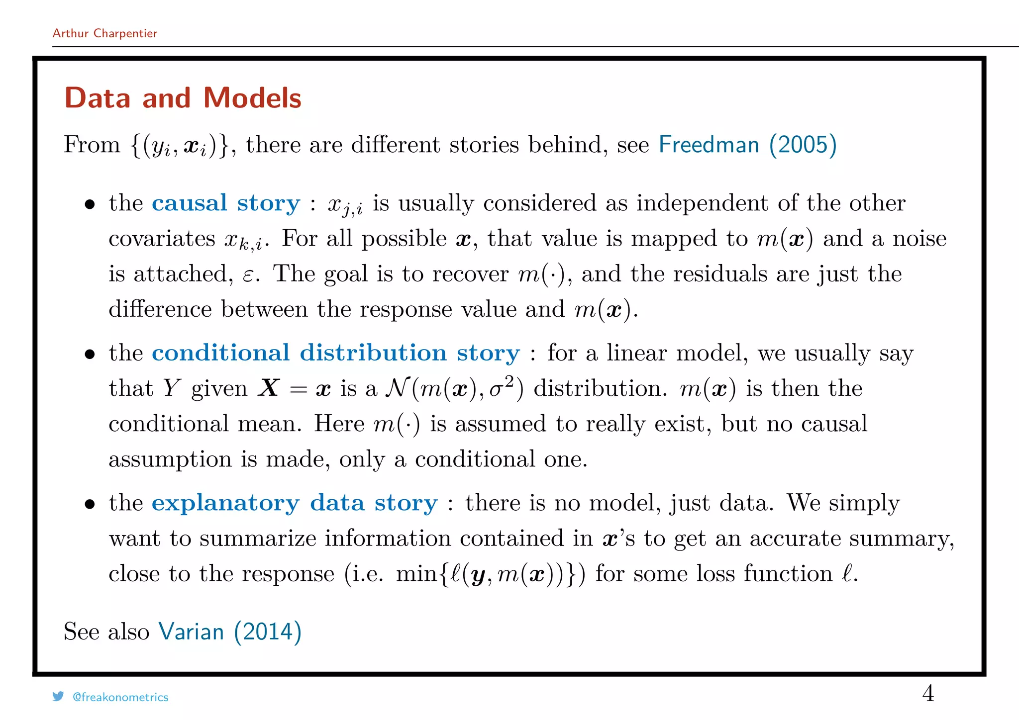
Data, Models & Causal Inference
We cannot differentiate data and model that easily..
After an operation, should I stay at hospital, or go back home ?
as in Angrist & Pischke (2008),
(health | hospital) − (health | stayed home) [observed]
should be written
(health | hospital) − (health | had stayed home) [treatment effect]
+ (health | had stayed home) − (health | stayed home) [selection bias]
Need randomization to solve selection bias.
@freakonometrics 5

6. Arthur Charpentier
Econometric Modeling
Data {(yi, xi)}, for i = 1, · · · , n, with xi ∈ X ⊂ Rp
and yi ∈ Y.
A model is a m : X → Y mapping
- regression, Y = R (but also Y = N)
- classification, Y = {0, 1}, {−1, +1}, {•, •}
(binary, or more)
Classification models are based on two steps,
• score function, s(x) = P(Y = 1|X = x) ∈ [0, 1]
• classifier s(x) → y ∈ {0, 1}.
q
q
q
q
q
q
q
q
q
q
0.0 0.2 0.4 0.6 0.8 1.0
0.00.20.40.60.81.0
q
q
q
q
q
q
q
q
q
q
@freakonometrics 6

7. Arthur Charpentier
High Dimensional Data (not to say ‘Big Data’)
See Bühlmann & van de Geer (2011) or Koch (2013), X is a n × p matrix
Portnoy (1988) proved that maximum likelihood estimators are asymptotically
normal when p2
/n → 0 as n, p → ∞. Hence, massive data, when p >
√
n.
More intersting is the sparcity concept, based not on p, but on the effective size.
Hence one can have p > n and convergent estimators.
High dimension might be scary because of curse of dimensionality, see
Bellman (1957). The volume of the unit sphere in Rp
tends to 0 as p → ∞,
i.e.space is sparse.
@freakonometrics 7

8. Arthur Charpentier
Computational & Nonparametric Econometrics
Linear Econometrics: estimate g : x → E[Y |X = x] by a linear function.
Nonlinear Econometrics: consider the approximation for some functional basis
g(x) =
∞
j=0
ωjgj(x) and g(x) =
h
j=0
ωjgj(x)
or a local model, on the neighborhood of x,
g(x) =
1
nx
i∈Ix
yi, with Ix = {x ∈ Rp
: xi−x ≤ h},
see Nadaraya (1964) and Watson (1964).
Here h is some tunning parameter: not estimated, but chosen (optimaly).
@freakonometrics 8

9. Arthur Charpentier
Econometrics & Probabilistic Model
from Cook & Weisberg (1999), see also Haavelmo (1965).
(Y |X = x) ∼ N(µ(x), σ2
) with µ(x) = β0 + xT
β, and β ∈ Rp
.
Linear Model: E[Y |X = x] = β0 + xT
β
Homoscedasticity: Var[Y |X = x] = σ2
.
@freakonometrics 9

10. Arthur Charpentier
Conditional Distribution and Likelihood
(Y |X = x) ∼ N(µ(x), σ2
) with µ(x) = β0 + xT
β, et β ∈ Rp
The log-likelihood is
log L(β0, β, σ2
|y, x) = −
n
2
log[2πσ2
] −
1
2σ2
n
i=1
(yi − β0 − xT
i β)2
.
Set
(β0, β, σ2
) = argmax log L(β0, β, σ2
|y, x) .
First order condition XT
[y − Xβ] = 0. If matrix X is a full rank matrix
β = (XT
X)−1
XT
y = β + (XT
X)−1
XT
ε.
Asymptotic properties of β,
√
n(β − β)
L
→ N(0, Σ) as n → ∞
@freakonometrics 10

11. Arthur Charpentier
Geometric Perspective
Define the orthogonal projection on X,
ΠX = X[XT
X]−1
XT
y = X[XT
X]−1
XT
ΠX
y = ΠXy.
Pythagoras’ theorem can be writen
y 2
= ΠXy 2
+ ΠX⊥ y 2
= ΠXy 2
+ y − ΠXy 2
which can be expressed as
n
i=1
y2
i
n×total variance
=
n
i=1
y2
i
n×explained variance
+
n
i=1
(yi − yi)2
n×residual variance
@freakonometrics 11

12. Arthur Charpentier
Geometric Perspective
Define the angle θ between y and ΠX y,
R2
=
ΠX y 2
y 2
= 1 −
ΠX⊥ y 2
y 2
= cos2
(θ)
see Davidson & MacKinnon (2003)
y = β0 + X1β1 + X2β2 + ε
If y2 = ΠX⊥
1
y and X2 = ΠX⊥
1
X2, then
β2 = [X2
T
X2]−1
X2
T
y2
X2 = X2 if X1 ⊥ X2,
Frisch-Waugh theorem.
@freakonometrics 12

13. Arthur Charpentier
From Linear to Non-Linear
y = Xβ = X[XT
X]−1
XT
H
y i.e. yi = hT
xi
y,
with - for the linear regression - hx = X[XT
X]−1
x.
One can consider some smoothed regression, see Nadaraya (1964) and Watson
(1964), with some smoothing matrix S
mh(x) = sT
xy =
n
i=1
sx,iyi withs sx,i =
Kh(x − xi)
Kh(x − x1) + · · · + Kh(x − xn)
for some kernel K(·) and some bandwidth h > 0.
@freakonometrics 13

14. Arthur Charpentier
From Linear to Non-Linear
T =
Sy − Hy
trace([S − H]T[S − H])
can be used to test for linearity, Simonoff (1996). trace(S) is the equivalent
number of parameters, and n − trace(S) the degrees of freedom, Ruppert et al.
(2003).
Nonlinear Model, but Homoscedastic - Gaussian
• (Y |X = x) ∼ N(µ(x), σ2
)
• E[Y |X = x] = µ(x)
@freakonometrics 14

15. Arthur Charpentier
Conditional Expectation
from Angrist & Pischke (2008), x → E[Y |X = x].
@freakonometrics 15

16. Arthur Charpentier
Exponential Distributions and Linear Models
f(yi|θi, φ) = exp
yiθi − b(θi)
a(φ)
+ c(yi, φ) with θi = h(xT
i β)
Log likelihood is expressed as
log L(θ, φ|y) =
n
i=1
log f(yi|θi, φ) =
n
i=1 yiθi −
n
i=1 b(θi)
a(φ)
+
n
i=1
c(yi, φ)
and first order conditions
∂ log L(θ, φ|y)
∂β
= XT
W −1
[y − µ] = 0
as in Müller (2001), where W is a weight matrix, function of β.
We usually specify the link function g(·) defined as
y = m(x) = E[Y |X = x] = g−1
(xT
β).
@freakonometrics 16

17. Arthur Charpentier
Exponential Distributions and Linear Models
Note that W = diag( g(y) · Var[y]), and set
z = g(y) + (y − y) · g(y)
the the maximum likelihood estimator is obtained iteratively
βk+1 = [XT
W −1
k X]−1
XT
W −1
k zk
Set β = β∞, so that
√
n(β − β)
L
→ N(0, I(β)−1
)
with I(β) = φ · [XT
W −1
∞ X].
Note that [XT
W −1
k X] is a p × p matrix.
@freakonometrics 17

18. Arthur Charpentier
Exponential Distributions and Linear Models
Generalized Linear Model:
• (Y |X = x) ∼ L(θx, ϕ)
• E[Y |X = x] = h−1
(θx) = g−1
(xT
β)
e.g. (Y |X = x) ∼ P(exp[xT
β]).
Use of maximum likelihood techniques for inference.
Actually, more a moment condition than a distribution assumption.
@freakonometrics 18

19. Arthur Charpentier
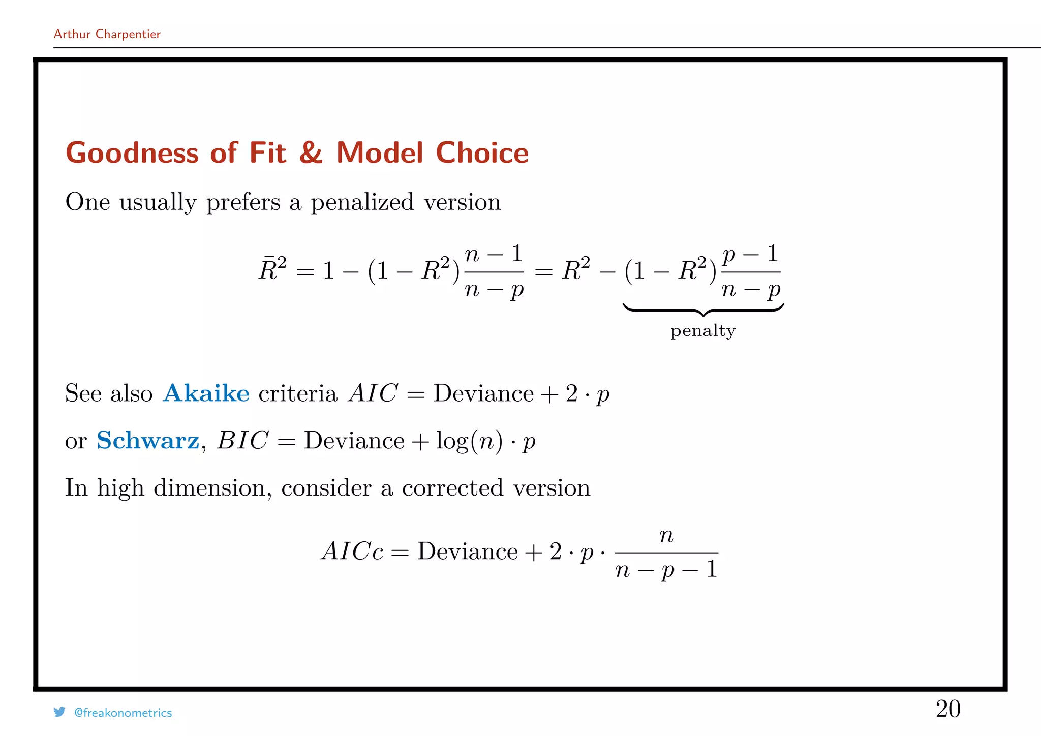
Goodness of Fit & Model Choice
From the variance decomposition
1
n
n
i=1
(yi − ¯y)2
total variance
=
1
n
n
i=1
(yi − yi)2
residual variance
+
1
n
n
i=1
(yi − ¯y)2
explained variance
and define
R2
=
n
i=1(yi − ¯y)2
−
n
i=1(yi − yi)2
n
i=1(yi − ¯y)2
More generally
Deviance(β) = −2 log[L] = 2
i=1
(yi − yi)2
= Deviance(y)
The null deviance is obtained using yi = y, so that
R2
=
Deviance(y) − Deviance(y)
Deviance(y)
= 1 −
Deviance(y)
Deviance(y)
= 1 −
D
D0
@freakonometrics 19

20. Arthur Charpentier
Goodness of Fit & Model Choice
One usually prefers a penalized version
¯R2
= 1 − (1 − R2
)
n − 1
n − p
= R2
− (1 − R2
)
p − 1
n − p
penalty
See also Akaike criteria AIC = Deviance + 2 · p
or Schwarz, BIC = Deviance + log(n) · p
In high dimension, consider a corrected version
AICc = Deviance + 2 · p ·
n
n − p − 1
@freakonometrics 20

21. Arthur Charpentier
Stepwise Procedures
Forward algorithm
1. set j1 = argmin
j∈{∅,1,··· ,n}
{AIC({j})}
2. set j2 = argmin
j∈{∅,1,··· ,n}{j1 }
{AIC({j1 , j})}
3. ... until j = ∅
Backward algorithm
1. set j1 = argmin
j∈{∅,1,··· ,n}
{AIC({1, · · · , n}{j})}
2. set j2 = argmin
j∈{∅,1,··· ,n}{j1 }
{AIC({1, · · · , n}{j1 , j})}
3. ... until j = ∅
@freakonometrics 21

22. Arthur Charpentier
Econometrics & Statistical Testing
Standard test for H0 : βk = 0 against H1 : βk = 0 is Student-t est tk = βk/seβk
,
Use the p-value P[|T| > |tk|] with T ∼ tν (and ν = trace(H)).
In high dimension, consider the FDR (False Discovery Ratio).
With α = 5%, 5% variables are wrongly significant.
If p = 100 with only 5 significant variables, one should expect also 5 false positive,
i.e. 50% FDR, see Benjamini & Hochberg (1995) and Andrew Gelman’s talk.
@freakonometrics 22

23. Arthur Charpentier
Under & Over-Identification
Under-identification is obtained when the true model is
y = β0 + xT
1 β1 + xT
2 β2 + ε, but we estimate y = β0 + xT
1 b1 + η.
Maximum likelihood estimator for b1 is
b1 = (XT
1 X1)−1
XT
1 y
= (XT
1 X1)−1
XT
1 [X1,iβ1 + X2,iβ2 + ε]
= β1 + (X1X1)−1
XT
1 X2β2
β12
+ (XT
1 X1)−1
XT
1 ε
νi
so that E[b1] = β1 + β12, and the bias is null when XT
1 X2 = 0 i.e. X1 ⊥ X2,
see Frisch-Waugh).
Over-identification is obtained when the true model is y = β0 + xT
1 β1ε, but we
fit y = β0 + xT
1 b1 + xT
2 b2 + η.
Inference is unbiased since E(b1) = β1 but the estimator is not efficient.
@freakonometrics 23

24. Arthur Charpentier
Statistical Learning & Loss Function
Here, no probabilistic model, but a loss function, . For some set of functions
M, X → Y, define
m = argmin
m∈M
n
i=1
(yi, m(xi))
Quadratic loss functions are interesting since
y = argmin
m∈R
n
i=1
1
n
[yi − m]2
which can be writen, with some underlying probabilistic model
E(Y ) = argmin
m∈R
Y − m 2
2
= argmin
m∈R
E [Y − m]2
For τ ∈ (0, 1), we obtain the quantile regression (see Koenker (2005))
m = argmin
m∈M0
n
i=1
τ (yi, m(xi)) avec τ (x, y) = |(x − y)(τ − 1x≤y)|
@freakonometrics 24

25. Arthur Charpentier
Boosting & Weak Learning
m = argmin
m∈M
n
i=1
(yi, m(xi))
is hard to solve for some very large and general space M of X → Y functions.
Consider some iterative procedure, where we learn from the errors,
m(k)
(·) = m1(·)
∼y
+ m2(·)
∼ε1
+ m3(·)
∼ε2
+ · · · + mk(·)
∼εk−1
= m(k−1)
(·) + mk(·).
Formely ε can be seen as , the gradient of the loss.
@freakonometrics 25

26. Arthur Charpentier
Boosting & Weak Learning
It is possible to see this algorithm as a gradient descent. Not
f(xk)
f,xk
∼ f(xk−1)
f,xk−1
+ (xk − xk−1)
αk
f(xk−1)
f,xk−1
but some kind of dual version
fk(x)
fk,x
∼ fk−1(x)
fk−1,x
+ (fk − fk−1)
ak
fk−1, x
where is a gradient is some functional space.
m(k)
(x) = m(k−1)
(x) + argmin
f∈F
n
i=1
(yi, m(k−1)
(x) + f(x))
for some simple space F so that we define some weak learner, e.g. step
functions (so called stumps)
@freakonometrics 26

27. Arthur Charpentier
Boosting & Weak Learning
Standard set F are stumps functions but one can also consider splines (with
non-fixed knots).
One might add a shrinkage parameter to learn even more weakly, i.e. set
ε1 = y − α · m1(x) with α ∈ (0, 1), etc.
@freakonometrics 27

28. Arthur Charpentier
Big Data & Linear Model
Consider some linear model yi = xT
i β + εi for all i = 1, · · · , n.
Assume that εi are i.i.d. with E(ε) = 0 (and finite variance). Write





y1
...
yn





y,n×1
=





1 x1,1 · · · x1,p
...
...
...
...
1 xn,1 · · · xn,p





X,n×(p+1)








β0
β1
...
βp








β,(p+1)×1
+





ε1
...
εn





ε,n×1
.
Assuming ε ∼ N(0, σ2
I), the maximum likelihood estimator of β is
β = argmin{ y − XT
β 2
} = (XT
X)−1
XT
y
... under the assumtption that XT
X is a full-rank matrix.
What if XT
X cannot be inverted? Then β = [XT
X]−1
XT
y does not exist, but
βλ = [XT
X + λI]−1
XT
y always exist if λ > 0.
@freakonometrics 28

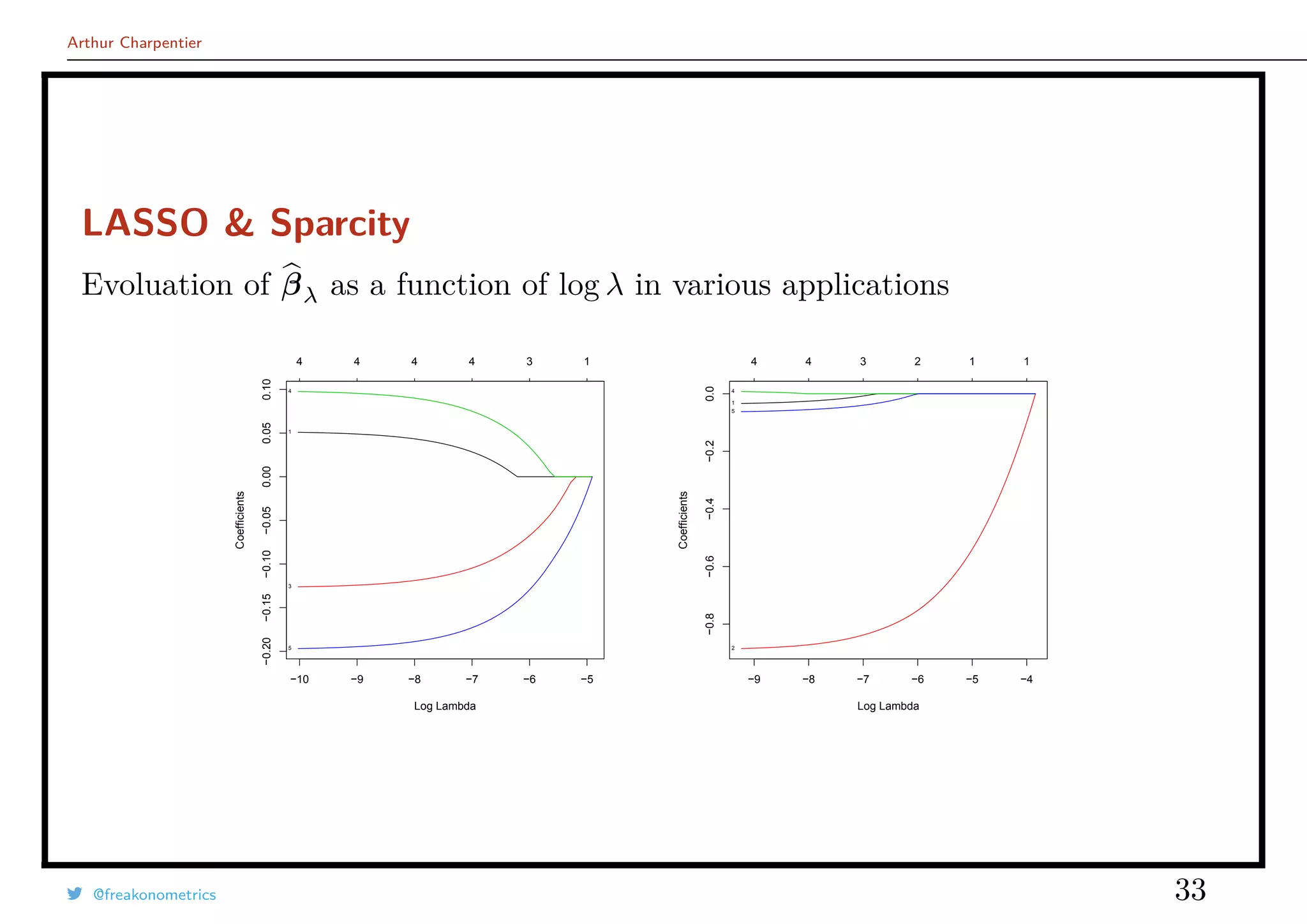
29. Arthur Charpentier
Ridge Regression & Regularization
The estimator β = [XT
X + λI]−1
XT
y is the Ridge estimate obtained as
solution of
β = argmin
β



n
i=1
[yi − β0 − xT
i β]2
+ λ β 2
2
1Tβ2



for some tuning parameter λ. One can also write
β = argmin
β; β 2 ≤s
{ Y − XT
β 2
}
There is a Bayesian interpretation of that regularization, when β has some prior
N(β0, τI).
@freakonometrics 29

30. Arthur Charpentier
Over-Fitting & Penalization
Solve here, for some norm · ,
min
n
i=1
(yi, β0 + xT
β) + λ β = min objective(β) + penality(β) .
Estimators are no longer unbiased, but might have a smaller mse.
Consider some i.id. sample {y1, · · · , yn} from N(θ, σ2
), and consider some
estimator proportional to y, i.e. θ = αy. α = 1 is the maximum likelihood
estimator.
Note that
mse[θ] = (α − 1)2
µ2
bias[θ]2
+
α2
σ2
n
Var[θ]
and α = µ2
· µ2
+
σ2
n
−1
< 1.
@freakonometrics 30

31. Arthur Charpentier
(β0, β) = argmin
n
i=1
(yi, β0 + xT
β) + λ β ,
can be seen as a Lagrangian minimization problem
(β0, β) = argmin
β; β ≤s
n
i=1
(yi, β0 + xT
β)
@freakonometrics 31

32. Arthur Charpentier
LASSO & Sparcity
In severall applications, p can be (very) large, but a lot of features are just noise:
βj = 0 for many j’s. Let s denote the number of relevent features, with
s << p, cf Hastie, Tibshirani & Wainwright (2015),
s = card{S} where S = {j; βj = 0}
The true model is now y = XT
SβS + ε, where XT
SXS is a full rank matrix.
@freakonometrics 32

33. Arthur Charpentier
LASSO & Sparcity
Evoluation of βλ as a function of log λ in various applications
−10 −9 −8 −7 −6 −5
−0.20−0.15−0.10−0.050.000.050.10
Log Lambda
Coefficients
4 4 4 4 3 1
1
3
4
5
−9 −8 −7 −6 −5 −4
−0.8−0.6−0.4−0.20.0 Log Lambda
Coefficients
4 4 3 2 1 1
1
2
4
5
@freakonometrics 33

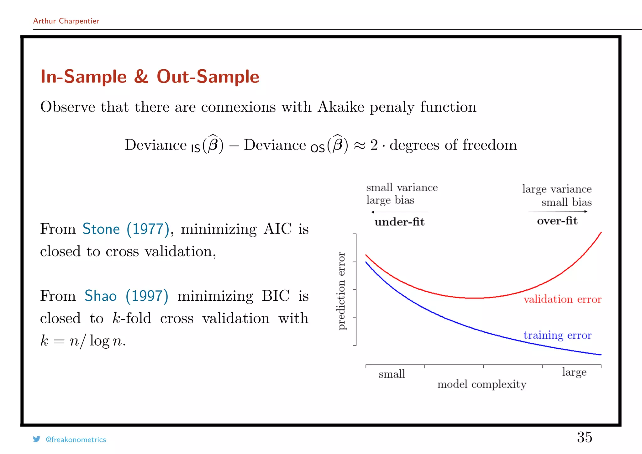
34. Arthur Charpentier
In-Sample & Out-Sample
Write β = β((x1, y1), · · · , (xn, yn)). Then (for the linear model)
Deviance IS(β) =
n
i=1
[yi − xT
i β((x1, y1), · · · , (xn, yn))]2
Withe this “in-sample” deviance, we cannot use the central limit theorem
Deviance IS(β)
n
→ E [Y − XT
β]
Hence, we can compute some “out-of-sample” deviance
Deviance OS(β) =
m+n
i=n+1
[yi − xT
i β((x1, y1), · · · , (xn, yn)]2
@freakonometrics 34

35. Arthur Charpentier
In-Sample & Out-Sample
Observe that there are connexions with Akaike penaly function
Deviance IS(β) − Deviance OS(β) ≈ 2 · degrees of freedom
From Stone (1977), minimizing AIC is
closed to cross validation,
From Shao (1997) minimizing BIC is
closed to k-fold cross validation with
k = n/ log n.
@freakonometrics 35

36. Arthur Charpentier
Overfit, Generalization & Model Complexity
Complexity of the model is the degree of the polynomial function
@freakonometrics 36

37. Arthur Charpentier
Cross-Validation
See Jacknife technique Quenouille (1956) or Tukey (1958) to reduce the bias.
If {y1, · · · , yn} is an i.id. sample from Fθ, with estimator Tn(y) = Tn(y1, · · · , yn),
such that E[Tn(Y )] = θ + O n−1
, consider
Tn(y) =
1
n
n
i=1
Tn−1(y(i)) avec y(i) = (y1, · · · , yi−1, yi+1, · · · , yn).
Then E[Tn(Y )] = θ + O n−2
.
Similar idea in leave-one-out cross validation
Risk =
1
n
n
i=1
(yi, m(i)(xi))
@freakonometrics 37

38. Arthur Charpentier
Rule of Thumb vs. Cross Validation
m[h ]
(x) = β
[x]
0 + β
[x]
1 x with (β
[x]
0 , β
[x]
1 ) = argmin
(β0,β1)
n
i=1
ω
[x]
h [yi − (β0 + β1xi)]2
q
q
q
q
q
q
q
q
q
q
q
q
q
q
q
q
q
q
q
q
q
q
q
q
q
q
q
qq
qq
q
q
q
q
q
q
q
q
q
q
qq
q
q
q
q
q
q
q
q
q
q
q
q
q
q
q
q
q
q
q
q
q
q
q
qq
q
q
q
q
q
qq
q
qq
q
q
q
q
q
q
q
q
q
q
q
q
q
q
q
q
q
q
q
q
q
q
0 2 4 6 8 10
−2−1012
set h = argmin mse(h) with mse(h) =
1
n
n
i=1
yi − m
[h]
(i)(xi)
2
@freakonometrics 38

39. Arthur Charpentier
Exponential Smoothing for Time Series
Consider some exponential smoothing filter, on a
time series (xt), yt+1 = αyt +(1−α)yt, then consider
α = argmin
T
t=2
(yt, yt) ,
see Hyndman et al. (2003).
@freakonometrics 39

40. Arthur Charpentier
Cross-Validation
Consider a partition of {1, · · · , n} in k groups with the same size, I1, · · · , Ik, and
set Ij = {1, · · · , n}Ij. Fit m(j) on Ij, and
Risk =
1
k
k
j=1
Riskj where Riskj =
k
n
i∈Ij
(yi, m(j)(xi))
@freakonometrics 40

41. Arthur Charpentier
Randomization is too important to be left to chance!
Consider some bootstraped sample, Ib = {i1,b, · · · , in,b}, with ik,b ∈ {1, · · · , n}
Set ni = 1i/∈I1
+ · · · + 1i/∈vB
, and fit mb on Ib
Risk =
1
n
n
i=1
1
ni
b:i/∈Ib
(yi, mb(xi))
Probability that ith obs. is not selection (1 − n−1
)n
→ e−1
∼ 36.8%,
see training / validation samples (2/3-1/3).
@freakonometrics 41

42. Arthur Charpentier
Bootstrap
From Efron (1987), generate samples from (Ω, F, Pn)
Fn(y) =
1
n
n
i=1
1(yi ≤ y) and Fn(yi) =
rank(yi)
n
.
If U ∼ U([0, 1]), F−1
(U) ∼ F
If U ∼ U([0, 1]), F−1
n (U) is uniform
on
1
n
, · · · ,
n − 1
n
, 1 .
Consider some boostraped sample,
- either (yik
, xik
), ik ∈ {1, · · · , n}
- or (yk + εik
, xk), ik ∈ {1, · · · , n}
@freakonometrics 42

43. Arthur Charpentier
Classification & Logistic Regression
Generalized Linear Model when Y has a Bernoulli distribution, yi ∈ {0, 1},
m(x) = E[Y |X = x] =
eβ0+xT
β
1 + eβ0+xTβ
= H(β0 + xT
β)
Estimate (β0, β) using maximum likelihood techniques
L =
n
i=1
exT
i β
1 + exT
i
β
yi
1
1 + exT
i
β
1−yi
Deviance ∝
n
i=1
log(1 + exT
i β
) − yixT
i β
Observe that
D0 ∝
n
i=1
[yi log(y) + (1 − yi) log(1 − y)]
@freakonometrics 43

44. Arthur Charpentier
Classification Trees
To split {N} into two {NL, NR}, consider
I(NL, NR) =
x∈{L,R}
nx
n
I(Nx)
e.g. Gini index (used originally in CART, see Breiman et al. (1984))
gini(NL, NR) = −
x∈{L,R}
nx
n
y∈{0,1}
nx,y
nx
1 −
nx,y
nx
and the cross-entropy (used in C4.5 and C5.0)
entropy(NL, NR) = −
x∈{L,R}
nx
n
y∈{0,1}
nx,y
nx
log
nx,y
nx
@freakonometrics 44

45. Arthur Charpentier
Classification Trees
1.0 1.5 2.0 2.5 3.0
−0.45−0.35−0.25
INCAR
15 20 25 30
−0.45−0.35−0.25
INSYS
12 16 20 24
−0.45−0.35−0.25
PRDIA
20 25 30 35
−0.45−0.35−0.25
PAPUL
4 6 8 10 12 14 16
−0.45−0.35−0.25
PVENT
500 1000 1500 2000
−0.45−0.35−0.25
REPUL
NL: {xi,j ≤ s} NR: {xi,j > s}
solve max
j∈{1,··· ,k},s
{I(NL, NR)}
←− first split
second split −→
1.8 2.2 2.6 3.0
−0.20−0.18−0.16−0.14
INCAR
20 24 28 32
−0.20−0.18−0.16−0.14
INSYS
12 14 16 18 20 22
−0.20−0.18−0.16−0.14
PRDIA
16 18 20 22 24 26 28
−0.20−0.18−0.16−0.14
PAPUL
4 6 8 10 12 14
−0.20−0.18−0.16−0.14
PVENT
500 700 900 1100
−0.20−0.18−0.16−0.14
REPUL
@freakonometrics 45

46. Arthur Charpentier
Trees & Forests
Boostrap can be used to define the concept of margin,
margini =
1
B
B
b=1
1(y
(b)
i = yi) −
1
B
B
b=1
1(y
(b)
i = yi)
Subsampling of variable, at each knot (e.g.
√
k out of k)
Concept of variable importance: given some random forest with M trees,
importance of variable k I(Xk) =
1
M m t
Nt
N
∆I(t)
where the first sum is over all trees, and the second one is over all nodes where
the split is done based on variable Xk.
@freakonometrics 46

47. Arthur Charpentier
Trees & Forests
0 5 10 15 20
50010001500200025003000
PVENT
REPUL
q
q
q
q
q
q
q
q
q
q
q
q
q qq
q
q
qq
q
q
q
q
q
q
q
q
q
q
q
q
q
q
q
q
q
q
q
q
q
q
q
q
q
q
q
q
q
q
q
q
q
q
q
q
q
q
q
q
q
q
q
q
q
q
q
q
q
q
q
q
See also discriminant analysis, SVM, neural networks, etc.
@freakonometrics 47

48. Arthur Charpentier
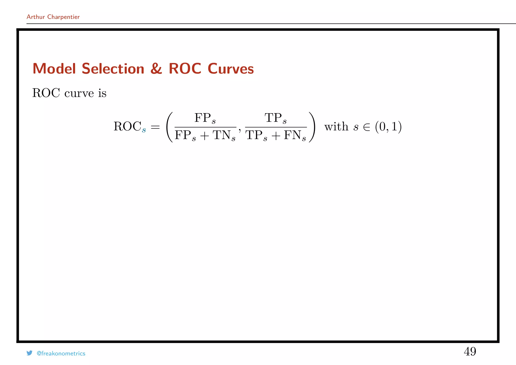
Model Selection & ROC Curves
Given a scoring function m(·), with m(x) = E[Y |X = x], and a threshold
s ∈ (0, 1), set
Y (s)
= 1[m(x) > s] =



1 if m(x) > s
0 if m(x) ≤ s
Define the confusion matrix as N = [Nu,v]
N(s)
u,v =
n
i=1
1(y
(s)
i = u, yj = v) for (u, v) ∈ {0, 1}.
Y = 0 Y = 1
Ys = 0 TNs FNs TNs+FNs
Ys = 1 FPs TPs FPs+TPs
TNs+FPs FNs+TPs n
@freakonometrics 48

49. Arthur Charpentier
Model Selection & ROC Curves
ROC curve is
ROCs =
FPs
FPs + TNs
,
TPs
TPs + FNs
with s ∈ (0, 1)
@freakonometrics 49

50. Arthur Charpentier
Model Selection & ROC Curves
In machine learning, the most popular measure is κ, see Landis & Koch (1977).
Define N⊥
from N as in the chi-square independence test. Set
total accuracy =
TP + TN
n
random accuracy =
TP⊥
+ TN⊥
n
=
[TN+FP] · [TP+FN] + [TP+FP] · [TN+FN]
n2
and
κ =
total accuracy − random accuracy
1 − random accuracy
.
See Kaggle competitions.
@freakonometrics 50

51. Arthur Charpentier
Reducing Dimension with PCA
Use principal components to reduce dimension (on centered and scaled
variables): we want d vectors z1, · · · , zd such that
First Compoment is z1 = Xω1 where
ω1 = argmax
ω =1
X · ω 2
= argmax
ω =1
ωT
XT
Xω
Second Compoment is z2 = Xω2 where
ω2 = argmax
ω =1
X
(1)
· ω 2
0 20 40 60 80
−8−6−4−2
Age
LogMortalityRate
−10 −5 0 5 10 15
−101234
PC score 1
PCscore2
q
q
qq
q
q
qqq
q
qqq
qq
q
qqq
q
q
q
qq
q
q
q
q
q
q
qqq
q
q
q
q
q
q
qq
q
qq
q
q
qq
q
q
q
q
q
q
qq
q
qqq
q
q
q
q
q
q
q
q
q
q
q
q
q
q
qq
q
q
qqq
q
qqq
qq
q
qqq
q
q
q
q
q
q
q
q
q
q
q
q
q
q
q
q
q
q
q
qq
q
q
q
q
qq
q
q
qq
q
q
qqqq
q
q
q
q
q
q
q
q
q
qqq
q
qqq
qq
q
qq
q
q
q
q
qq
q
q
q
q
q
q
q
q
q
q
q
q
q
1914
1915
1916
1917
1918
1919
1940
1942
1943
1944
0 20 40 60 80
−10−8−6−4−2
Age
LogMortalityRate
−10 −5 0 5 10 15
−10123
PC score 1
PCscore2
qq
q
q
q
q
q
qq
qq
qq
q
q
q
q
q
q
q
q
q
q
q
q
q
q
q
q
q
q
q
q
q
q
q
q
q
q
q
q
q
qq
qq
q
q
q
q
q
qq
q
q
q
q
q
q
q
q
q
q
q
q
q
q
q
q
q
q
q
q
q
q
q
q
q
q
qq
qq
q
q
q
q
q
q
q
q
q
q
q
q
q
q
q
q
q
q
q
q
q
qq
q
q
q
q
q
q
qq
q
q
q
q
q
q
q
q
q
qq
q
q
q
q
q
q
q
q
q
q
qq
qq
q
q
q
q
q
qq
qqqq
q
qqqq
q
q
q
q
q
q
with X
(1)
= X − Xω1
z1
ωT
1 .
@freakonometrics 51

52. Arthur Charpentier
Reducing Dimension with PCA
A regression on (the d) principal components, y = zT
b + η could be an
interesting idea, unfortunatley, principal components have no reason to be
correlated with y. First compoment was z1 = Xω1 where
ω1 = argmax
ω =1
X · ω 2
= argmax
ω =1
ωT
XT
Xω
It is a non-supervised technique.
Instead, use partial least squares, introduced in Wold (1966). First
compoment is z1 = Xω1 where
ω1 = argmax
ω =1
{< y, X · ω >} = argmax
ω =1
ωT
XT
yyT
Xω
(etc.)
@freakonometrics 52

53. Arthur Charpentier
Instrumental Variables
Consider some instrumental variable model, yi = xT
i β + εi such that
E[Yi|Z] = E[Xi|Z]T
β + E[εi|Z]
The estimator of β is
βIV = [ZT
X]−1
ZT
y
If dim(Z) > dim(X) use the Generalized Method of Moments,
βGMM = [XT
ΠZX]−1
XT
ΠZy with ΠZ = Z[ZT
Z]−1
ZT
@freakonometrics 53

54. Arthur Charpentier
Instrumental Variables
Consider a standard two step procedure
1) regress colums of X on Z, X = Zα + η, and derive predictions X = ΠZX
2) regress Y on X, yi = xT
i β + εi, i.e.
βIV = [ZT
X]−1
ZT
y
See Angrist & Krueger (1991) with 3 up to 1530 instruments : 12 instruments
seem to contain all necessary information.
Use LASSO to select necessary instruments, see Belloni, Chernozhukov & Hansen
(2010)
@freakonometrics 54

55. Arthur Charpentier
Take Away Conclusion
Big data mythology
- n → ∞: 0/1 law, everything is simplified (either true or false)
- p → ∞: higher algorithmic complexity, need variable selection tools
Econometrics vs. Machine Learning
- probabilistic interpretation of econometric models
(unfortunately sometimes misleading, e.g. p-value)
can deal with non-i.id data (time series, panel, etc)
- machine learning is about predictive modeling and generalization
algorithmic tools, based on bootstrap (sampling and sub-sampling),
cross-validation, variable selection, nonlinearities, cross effects, etc
Importance of visualization techniques (forgotten in econometrics publications)
@freakonometrics 55