Download as PDF, PPTX


![Arthur CHARPENTIER, Econometrics & “Machine Learning”, May 2018, Università degli studi dell’Insubria
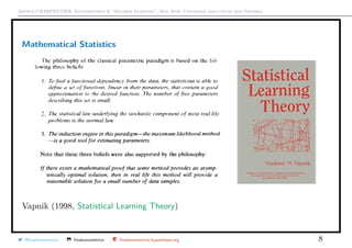
Conditional Distributions and Likelihood
We had a sample {y1, · · · , yn}, with Y from a N(θ, σ2
) distribution.
The natural extension if we had a sample {(y1, x1), · · · , (yn, xn)} is to assume
that Y |X = x has a N(θx, σ2
) distribution.
The standard linear model is obtained when θx is linear, θx = β0 + xT
β. Hence
E[Y |X = x] = xT
β and Var[Y |X = x] = σ2
(homoskedasticity).
(if we center variables or if we add the constant in x).
The MLE of β is
β
mle
= argmin
n
i=1
(yi − xi
T
β)2
= (XT
X)−1
XT
y.
@freakonometrics freakonometrics freakonometrics.hypotheses.org 12](https://image.slidesharecdn.com/vareseitalieseminar-180501103435/85/Varese-italie-seminar-12-320.jpg)
![Arthur CHARPENTIER, Econometrics & “Machine Learning”, May 2018, Università degli studi dell’Insubria
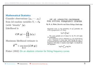
From a Gaussian to a Bernoulli (Logistic) Regression, and GLMs
Consider y ∈ {0, 1}, so that Y has a Bernoulli distribution. The logarithm of the
odds is linear,
log
P[Y = 1|X = x]
P[Y = 1|X = x]
= β0 + xT
β,
i.e.
E[Y |X = x] =
eβ0+xT
β
1 + eβ0+xTβ
= H(β0 + xT
β), où H(·) =
exp(·)
1 + exp(·)
,
with likelihood
L(β; y, X) =
n
i=1
exT
i β
1 + exT
i
β
yi
1
1 + exT
i
β
1−yi
and set β
mle
= arg max
β∈Rp
{L(β; y, X)} (solved numerically).
@freakonometrics freakonometrics freakonometrics.hypotheses.org 13](https://image.slidesharecdn.com/vareseitalieseminar-180501103435/85/Varese-italie-seminar-13-320.jpg)
![Arthur CHARPENTIER, Econometrics & “Machine Learning”, May 2018, Università degli studi dell’Insubria
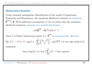
A Brief Excursion to Nonparametric Econometrics
Two strategies are usually considered to compute m(x) = E[Y |X = x]
• consider a local approximation (in the neighborhood of x), e.g. k-nearest
neighbor, kernel regression, lowess
• consider a functional decomposition of function m in some natural basis, e.g.
splines
For a kernel regression, as in Nadaraya (1964, ) and Watson (1964, ), consider
some kernel function K and some bandwidth h
mh(x) = sx
T
y =
n
i=1
sx,iyi where sx,i =
Kh(x − xi)
Kh(x − x1) + · · · + Kh(x − xn)
.
(in a univariate problem).
@freakonometrics freakonometrics freakonometrics.hypotheses.org 14](https://image.slidesharecdn.com/vareseitalieseminar-180501103435/85/Varese-italie-seminar-14-320.jpg)
![Arthur CHARPENTIER, Econometrics & “Machine Learning”, May 2018, Università degli studi dell’Insubria
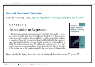
A Brief Excursion to Nonparametric Econometrics
Recall - see Simonoff (1996, ) that using asymtptotic approximations
bias[mh(x)] = E[mh(x)] − m(x) ∼ h2 C1
2
m (x) + C2m (x)
f (x)
f(x)
Var[mh(x)] ∼
C3
nh
σ(x)
f(x)
for some constants C1, C2 and C3.
Set mse[mh(x)] = bias2
[mh(x)] + Var[mh(x)] and consider the integrated version
mise[mh] = mse[mh(x)]dF(x)
@freakonometrics freakonometrics freakonometrics.hypotheses.org 15](https://image.slidesharecdn.com/vareseitalieseminar-180501103435/85/Varese-italie-seminar-15-320.jpg)
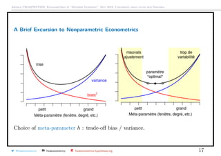
![Arthur CHARPENTIER, Econometrics & “Machine Learning”, May 2018, Università degli studi dell’Insubria
A Brief Excursion to Nonparametric Econometrics
mise[mh] ∼
bias2
h4
4
x2
k(x)dx
2
m (x) + 2m (x)
f (x)
f(x)
2
dx
+
variance
σ2
nh
k2
(x)dx ·
dx
f(x)
,
Thus, the optimal value is h = O(n−1/5
) (see Silverman’s rule of thumb).
Obtained using asymptotic theory and approximations.
@freakonometrics freakonometrics freakonometrics.hypotheses.org 16](https://image.slidesharecdn.com/vareseitalieseminar-180501103435/85/Varese-italie-seminar-16-320.jpg)
![Arthur CHARPENTIER, Econometrics & “Machine Learning”, May 2018, Università degli studi dell’Insubria
Model (and Variable) Choice
Suppose that the true model is yi = x1,iβ1 + x2,iβ2 + εi, but we estimate the
model on x1 (only) yi = X1,ib1 + ηi.
b1 = (XT
1 X1)−1
XT
1 Y
= (XT
1 X1)−1
XT
1 [X1,iβ1 + X2,iβ2 + ε]
= (XT
1 X1)−1
XT
1 X1β1 + (XT
1 X1)−1
XT
1 X2β2 + (XT
1 X1)−1
XT
1 ε
= β1 + (X1X1)−1
XT
1 X2β2
β12
+ (XT
1 X1)−1
XT
1 εi
νi
i.e. E(b1) = β1 + β12. If XT
1 X2 = 0 (X1 ⊥ X2), E(b1) = β1
Conversely, assume that the true model is yi = x1,iβ1 + εi but we estimated on
(unnecessary) variables X2 yi = x1,ib1 + x2,ib2 + ηi. Here estimation is unbiased
E(b1) = β1, but the estimator is not efficient...
@freakonometrics freakonometrics freakonometrics.hypotheses.org 18](https://image.slidesharecdn.com/vareseitalieseminar-180501103435/85/Varese-italie-seminar-18-320.jpg)
![Arthur CHARPENTIER, Econometrics & “Machine Learning”, May 2018, Università degli studi dell’Insubria
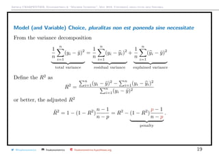
Model (and Variable) Choice, pluralitas non est ponenda sine necessitate
Alternative approach on penalization : consider a linear predictor m ∈ M
M = m : m(x) = sh(x)T
y where S = (s(x1), · · · , s(xn))T
smoothing matrix
Suppose that the true model is y = m0(x) + ε with E[ε] = 0 and Var[ε] = σ2
I, so
that m0(x) = E[Y |X = x]. Quadratic risk R(m) = E (Y − m(X))2
is
E (Y − m0(X))2
error
+ E (m0(X) − E[m(X)])2
bias2
+ E (E[m(X)] − m(X))2
variance
.
Consider empirical risk, Rn(m) =
1
n
n
i=1
(yi − m(xi))2
, then one can prove that
R(m) = E Rn(m) +
2σ2
n
trace(S),
see Mallow’s Cp from Mallow (1973, Some Comments on Cp)
@freakonometrics freakonometrics freakonometrics.hypotheses.org 21](https://image.slidesharecdn.com/vareseitalieseminar-180501103435/85/Varese-italie-seminar-21-320.jpg)

![Arthur CHARPENTIER, Econometrics & “Machine Learning”, May 2018, Università degli studi dell’Insubria
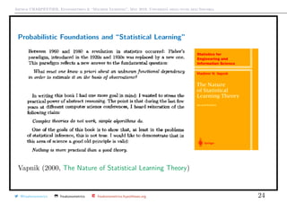
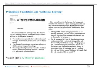
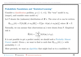
Probabilistic Foundations and “Statistical Learning”
Suppose that M contains a finite number of models. For any , δ, P and m0, if
we have enough observations ( n ≥ −1
log[δ−1
M ]), if
m ∈ argmin
m∈M
1
n
n
i=1
1(m(xi) = yi)
then with probability higher than 1 − δ, RP,f (m ) ≤ .
Here nM( , δ) = −1
log[δ−1
M ] is called complexity, and M is PAC-learnable.
If M is not finite, the problem is more complicated, it is necessary to define a
dimension d - so called VC-dimension - of M, that will be a substitute to M .
@freakonometrics freakonometrics freakonometrics.hypotheses.org 27](https://image.slidesharecdn.com/vareseitalieseminar-180501103435/85/Varese-italie-seminar-27-320.jpg)
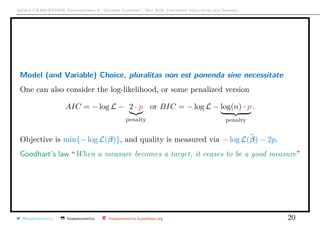
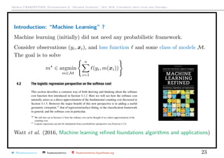
![Arthur CHARPENTIER, Econometrics & “Machine Learning”, May 2018, Università degli studi dell’Insubria
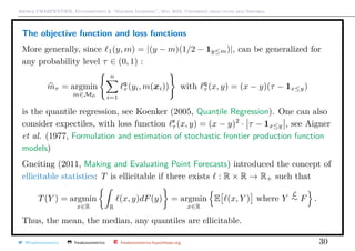
The objective function and loss functions
Consider loss function : Y × Y → R+ and set m ∈ argmin
m∈M
n
i=1
(yi, m(xi)) .
A classical loss function is the quadratic one 2(u, v) = (u − v)2
. Recall that
y = argmin
m∈R
n
i=1
2(yi, m) , or (for the continuous version)
E(Y ) = argmin
m∈R
Y − m 2
2
= argmin
m∈R
E 2(Y, m) .
One can also consider the least absolute value one 1(u, v) = |u − v. Recall that
median[y] = argmin
m∈R
n
i=1
1(yi, m) . The optimisation problem
m = argmin
m∈M
n
i=1
|yi − m(xi)|
is well know in robust econometrics.
@freakonometrics freakonometrics freakonometrics.hypotheses.org 29](https://image.slidesharecdn.com/vareseitalieseminar-180501103435/85/Varese-italie-seminar-29-320.jpg)
![Arthur CHARPENTIER, Econometrics & “Machine Learning”, May 2018, Università degli studi dell’Insubria
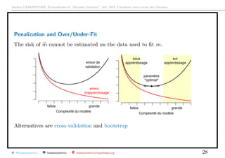
Penalization and Over/Under-Fit
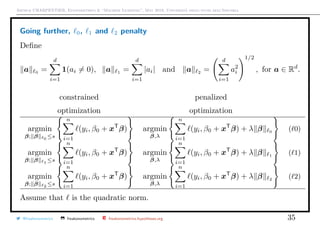
Consider some penalized objective function, given λ ≥ 0,
(β0,λ, βλ) = argmin
n
i=1
(yi, β0 + xT
β) + λ β
with centered and scaled variables, for some penalty β .
Note that there is some Bayesian interpretation
P[θ|y]
a posteriori
∝ P[y|θ]
likelihood
· P[θ]
a priori
i.e. log P[θ|y] = log P[y|θ]
log likelihood
+ log P[θ]
penalization
.
@freakonometrics freakonometrics freakonometrics.hypotheses.org 34](https://image.slidesharecdn.com/vareseitalieseminar-180501103435/85/Varese-italie-seminar-34-320.jpg)
![Arthur CHARPENTIER, Econometrics & “Machine Learning”, May 2018, Università degli studi dell’Insubria
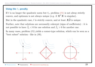
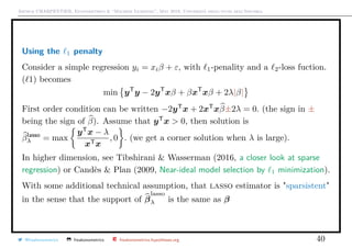
Using the 0 penalty
Foster & George (1994, the risk inflation criterion for multiple regression) tried to
solve directly the penalized problem of ( 0).
But it is a complex combinatorial problem in high dimension (Natarajan (1995)
sparse approximate solutions to linear systems proved that it was a NP-hard
problem)
One can prove that if λ ∼ σ2
log(p), alors
E [xT
β − xT
β0]2
≤ E [xS
T
βS − xT
β0]2
=σ2#S
· 4 log p + 2 + o(1) .
In that case
β
sub
λ,j =
0 si j /∈ Sλ(β)
β
ols
j si j ∈ Sλ(β),
where Sλ(β) is the set of non-null values in solutions of ( 0).
@freakonometrics freakonometrics freakonometrics.hypotheses.org 37](https://image.slidesharecdn.com/vareseitalieseminar-180501103435/85/Varese-italie-seminar-37-320.jpg)
![Arthur CHARPENTIER, Econometrics & “Machine Learning”, May 2018, Università degli studi dell’Insubria
Using the 2 penalty
With the 2-norm, ( 2) is the Ridge regression
β
ridge
λ = (XT
X + λI)−1
XT
y = (XT
X + λI)−1
(XT
X)β
ols
.
see Tikhonov (1943, On the stability of inverse problems). Hence
biais[β
ridge
λ ] = −λ[XT
X+λI]−1
β
ols
, Var[β
ridge
λ ] = σ2
[XT
X+λI]−1
XT
X[XT
X+λI]−1
.
With orthogonal variables (i.e. XT
X = I), we get
biais[β
ridge
λ ] =
λ
1 + λ
β
ols
and Var[β
ridge
λ ] =
σ2
(1 + λ)2
I =
Var[β
ols
]
(1 + λ)2
.
Note thatVar[β
ridge
λ ] < Var[β
ols
]. Further, mse[β
ridge
λ ] is minimal when
λ = pσ2
/βT
β.
@freakonometrics freakonometrics freakonometrics.hypotheses.org 38](https://image.slidesharecdn.com/vareseitalieseminar-180501103435/85/Varese-italie-seminar-38-320.jpg)
![Arthur CHARPENTIER, Econometrics & “Machine Learning”, May 2018, Università degli studi dell’Insubria
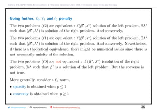
Going further, 0, 1 and 2 penalty
Thus, lasso can be used for variable selection (see Hastie et al. (2001 The
Elements of Statistical Learning).
With orthonormal covariance, one can prove that
βsub
λ,j = βols
j 1|βsub
λ,j
|>b
, βridge
λ,j =
βols
j
1 + λ
and βlasso
λ,j = sign[βols
j ] · (|βols
j | − λ)+.
@freakonometrics freakonometrics freakonometrics.hypotheses.org 41](https://image.slidesharecdn.com/vareseitalieseminar-180501103435/85/Varese-italie-seminar-41-320.jpg)
![Arthur CHARPENTIER, Econometrics & “Machine Learning”, May 2018, Università degli studi dell’Insubria
Econometric Modeling
Data {(yi, xi)}, for i = 1, · · · , n, with xi ∈ X ⊂ Rp
and yi ∈ Y.
A model is a m : X → Y mapping
- regression, Y = R (but also Y = N)
- classification, Y = {0, 1}, {−1, +1}, {•, •}
(binary, or more)
Classification models are based on two steps,
• score function, s(x) = P(Y = 1|X = x) ∈ [0, 1]
• classifier s(x) → y ∈ {0, 1}.
q
q
q
q
q
q
q
q
q
q
0.0 0.2 0.4 0.6 0.8 1.0
0.00.20.40.60.81.0
q
q
q
q
q
q
q
q
q
q
@freakonometrics freakonometrics freakonometrics.hypotheses.org 42](https://image.slidesharecdn.com/vareseitalieseminar-180501103435/85/Varese-italie-seminar-42-320.jpg)
![Arthur CHARPENTIER, Econometrics & “Machine Learning”, May 2018, Università degli studi dell’Insubria
Model Selection & ROC Curves
Given a scoring function m(·), with m(x) = E[Y |X = x], and a threshold
s ∈ (0, 1), set
Y (s)
= 1[m(x) > s] =
1 if m(x) > s
0 if m(x) ≤ s
Define the confusion matrix as N = [Nu,v]
Y = 0 Y = 1
Ys = 0 TNs FNs TNs+FNs
Ys = 1 FPs TPs FPs+TPs
TNs+FPs FNs+TPs n
ROC curve is
ROCs =
FPs
FPs + TNs
,
TPs
TPs + FNs
with s ∈ (0, 1)
@freakonometrics freakonometrics freakonometrics.hypotheses.org 44](https://image.slidesharecdn.com/vareseitalieseminar-180501103435/85/Varese-italie-seminar-44-320.jpg)
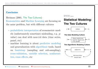

This document summarizes a seminar on econometrics and machine learning given by Arthur Charpentier at Università degli studi dell’Insubria in May 2018. It discusses the history and development of econometrics, including its probabilistic foundations. It also covers key econometric techniques like regression, maximum likelihood estimation, and nonparametric methods. Model selection criteria like AIC and BIC are also briefly discussed. The document provides a high-level overview of major topics in econometrics through the lens of its use in large datasets and connection to machine learning.