Download to read offline
![Arthur CHARPENTIER - Probit transformation for nonparametric kernel estimation of the copula
Motivation
Consider some n-i.i.d. sample {(Xi, Yi)} with cu-
mulative distribution function FXY and joint den-
sity fXY . Let FX and FY denote the marginal
distributions, and C the copula,
FXY (x, y) = C(FX(x), FY (y))
so that
fXY (x, y) = fX(x)fY (y)c(FX(x), FY (y))
We want a nonparametric estimate of c on [0, 1]2
. 1e+01 1e+03 1e+05
1e+011e+021e+031e+041e+05
2](https://image.slidesharecdn.com/slides-cirm-2016-light-160208151543/75/slides-CIRM-copulas-extremes-and-actuarial-science-2-2048.jpg)
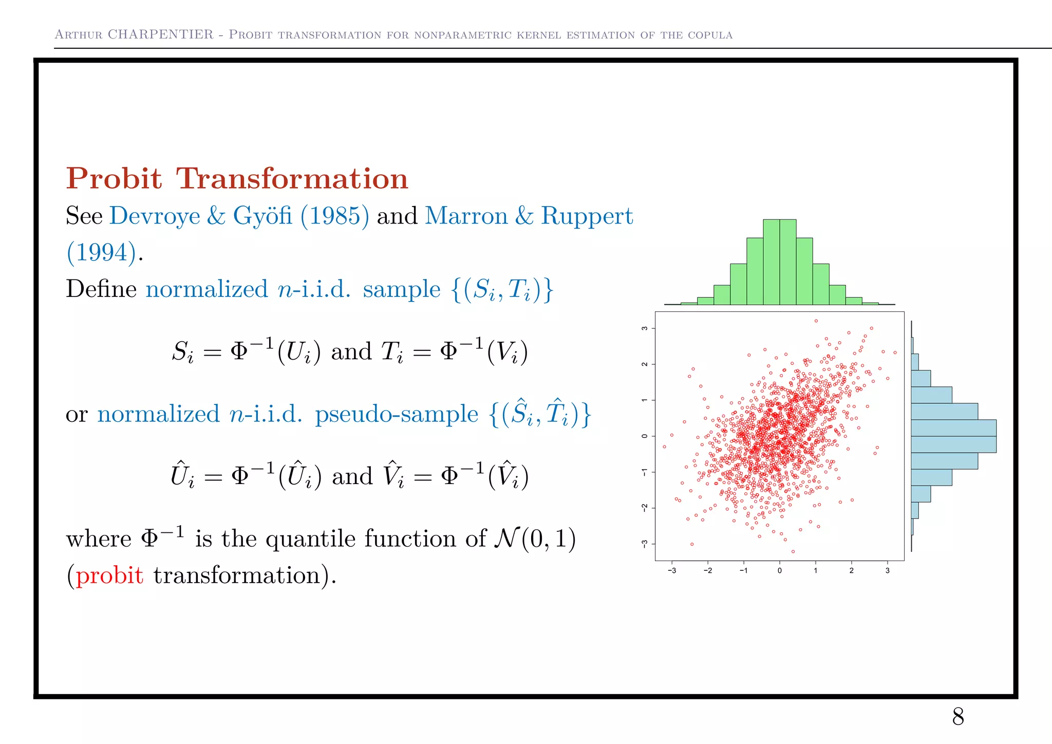
![Arthur CHARPENTIER - Probit transformation for nonparametric kernel estimation of the copula
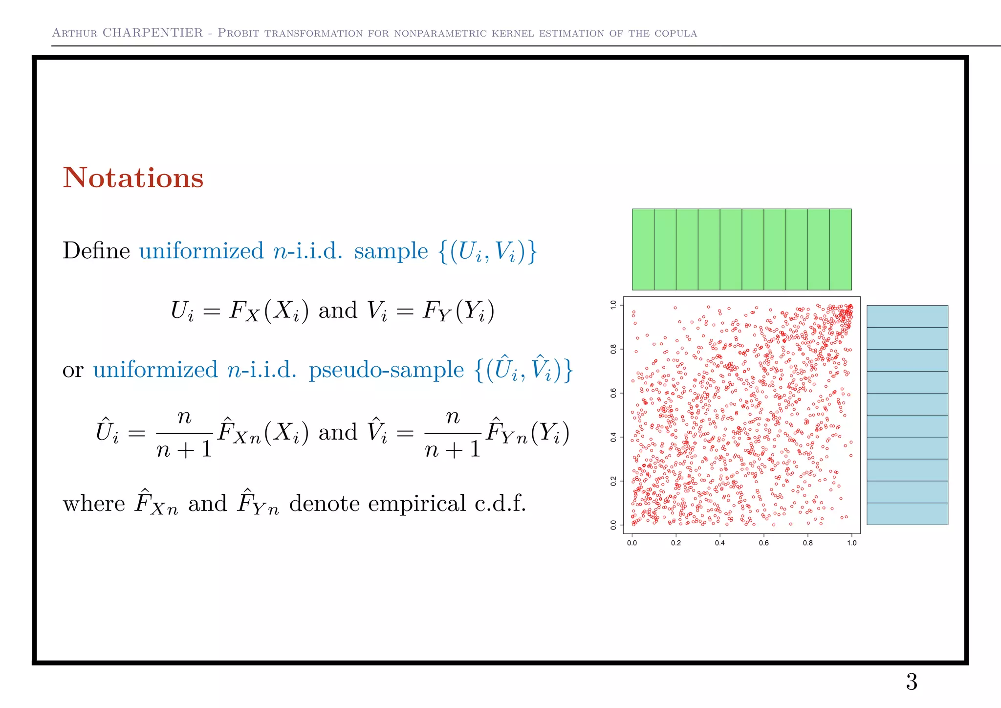
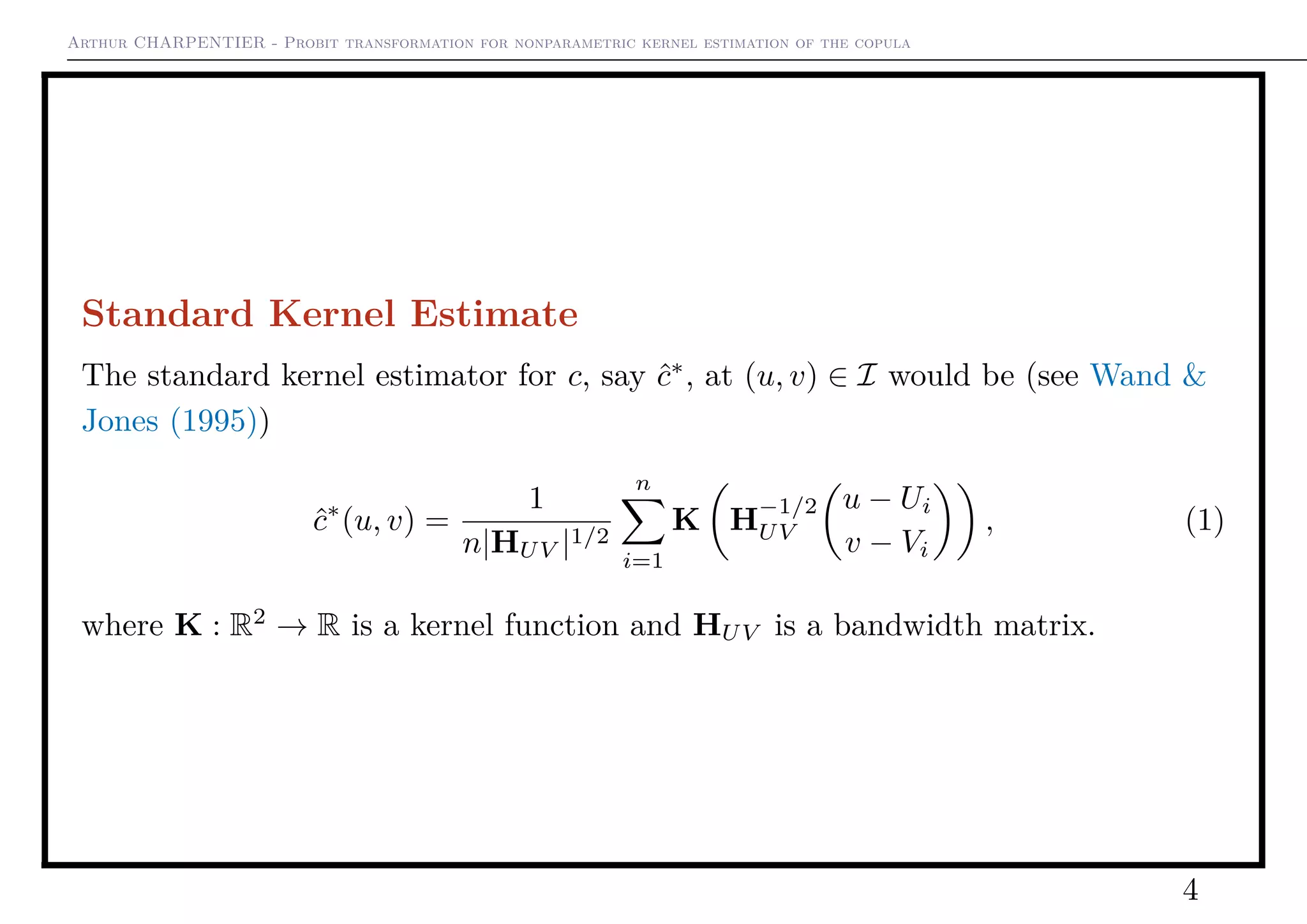
Standard Kernel Estimate
However, this estimator is not consistent along
boundaries of [0, 1]2
E(ˆc∗
(u, v)) =
1
4
c(u, v) + O(h) at corners
E(ˆc∗
(u, v)) =
1
2
c(u, v) + O(h) on the borders
if K is symmetric and HUV symmetric.
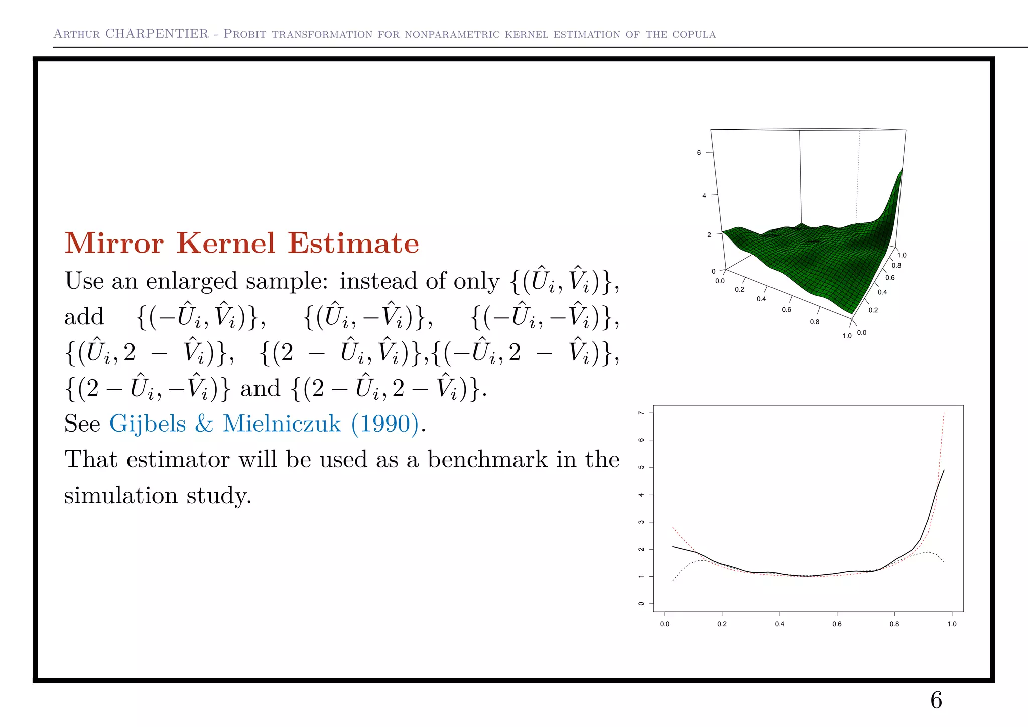
Corrections have been proposed, e.g. mirror reflec-
tion Gijbels (1990) or the usage of boundary kernels
Chen (2007), but with mixed results.
Remark: the graph on the bottom is ˆc∗
on the
(first) diagonal.
0.0
0.2
0.4
0.6
0.8
1.0 0.0
0.2
0.4
0.6
0.8
1.0
0
2
4
6
0.0 0.2 0.4 0.6 0.8 1.0
01234567
5](https://image.slidesharecdn.com/slides-cirm-2016-light-160208151543/75/slides-CIRM-copulas-extremes-and-actuarial-science-5-2048.jpg)
![Arthur CHARPENTIER - Probit transformation for nonparametric kernel estimation of the copula
Using Beta Kernels
Use a Kernel which is a product of beta kernels
Kxi
(u)) ∝ u
x1,i
b
1 [1 − u1]
x1,i
b · u
x2,i
b
2 [1 − u2]
x2,i
b
See Chen (1999).
0.0
0.2
0.4
0.6
0.8
1.0 0.0
0.2
0.4
0.6
0.8
1.0
0
2
4
6
0.0 0.2 0.4 0.6 0.8 1.0
01234567
7](https://image.slidesharecdn.com/slides-cirm-2016-light-160208151543/75/slides-CIRM-copulas-extremes-and-actuarial-science-7-2048.jpg)
![Arthur CHARPENTIER - Probit transformation for nonparametric kernel estimation of the copula
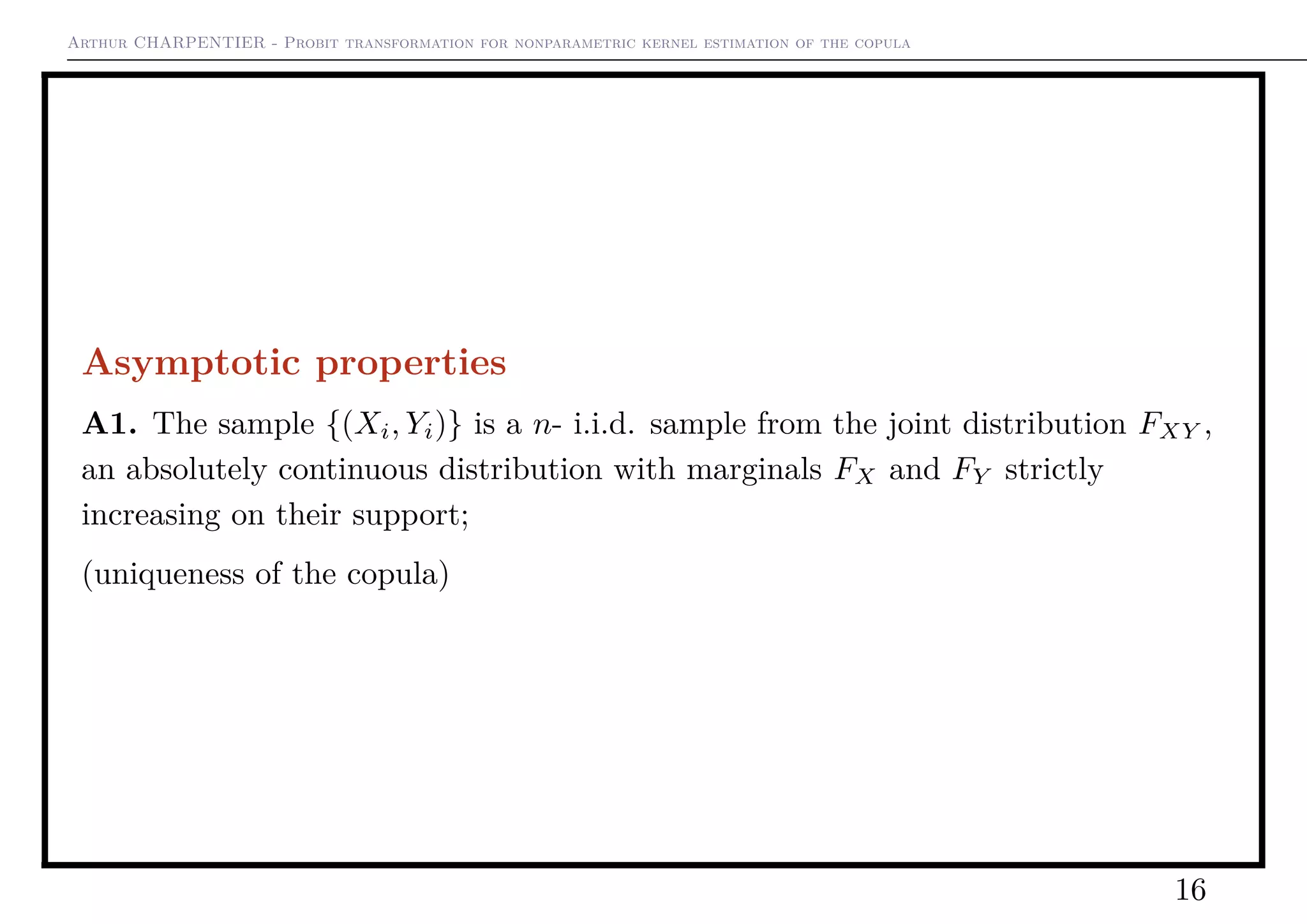
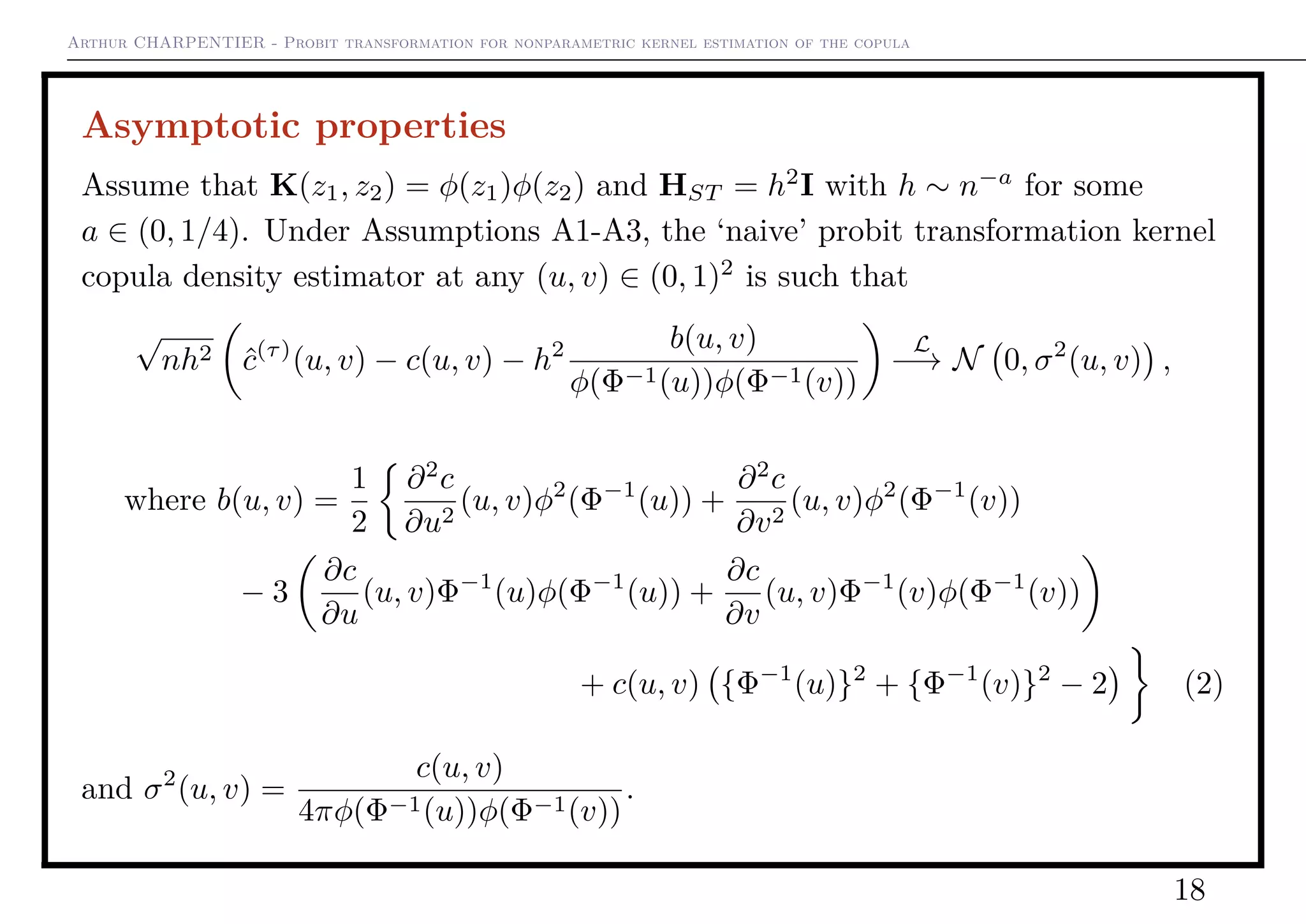
Asymptotic properties
A2. The copula C of FXY is such that (∂C/∂u)(u, v) and (∂2
C/∂u2
)(u, v) exist
and are continuous on {(u, v) : u ∈ (0, 1), v ∈ [0, 1]}, and (∂C/∂v)(u, v) and
(∂2
C/∂v2
)(u, v) exist and are continuous on {(u, v) : u ∈ [0, 1], v ∈ (0, 1)}. In
addition, there are constants K1 and K2 such that
∂2
C
∂u2
(u, v) ≤
K1
u(1 − u)
for (u, v) ∈ (0, 1) × [0, 1];
∂2
C
∂v2
(u, v) ≤
K2
v(1 − v)
for (u, v) ∈ [0, 1] × (0, 1);
A3. The density c of C exists, is positive and admits continuous second-order
partial derivatives on the interior of the unit square I. In addition, there is a
constant K00 such that
c(u, v) ≤ K00 min
1
u(1 − u)
,
1
v(1 − v)
∀(u, v) ∈ (0, 1)2
.
see Segers (2012).
17](https://image.slidesharecdn.com/slides-cirm-2016-light-160208151543/75/slides-CIRM-copulas-extremes-and-actuarial-science-17-2048.jpg)
![Arthur CHARPENTIER - Probit transformation for nonparametric kernel estimation of the copula
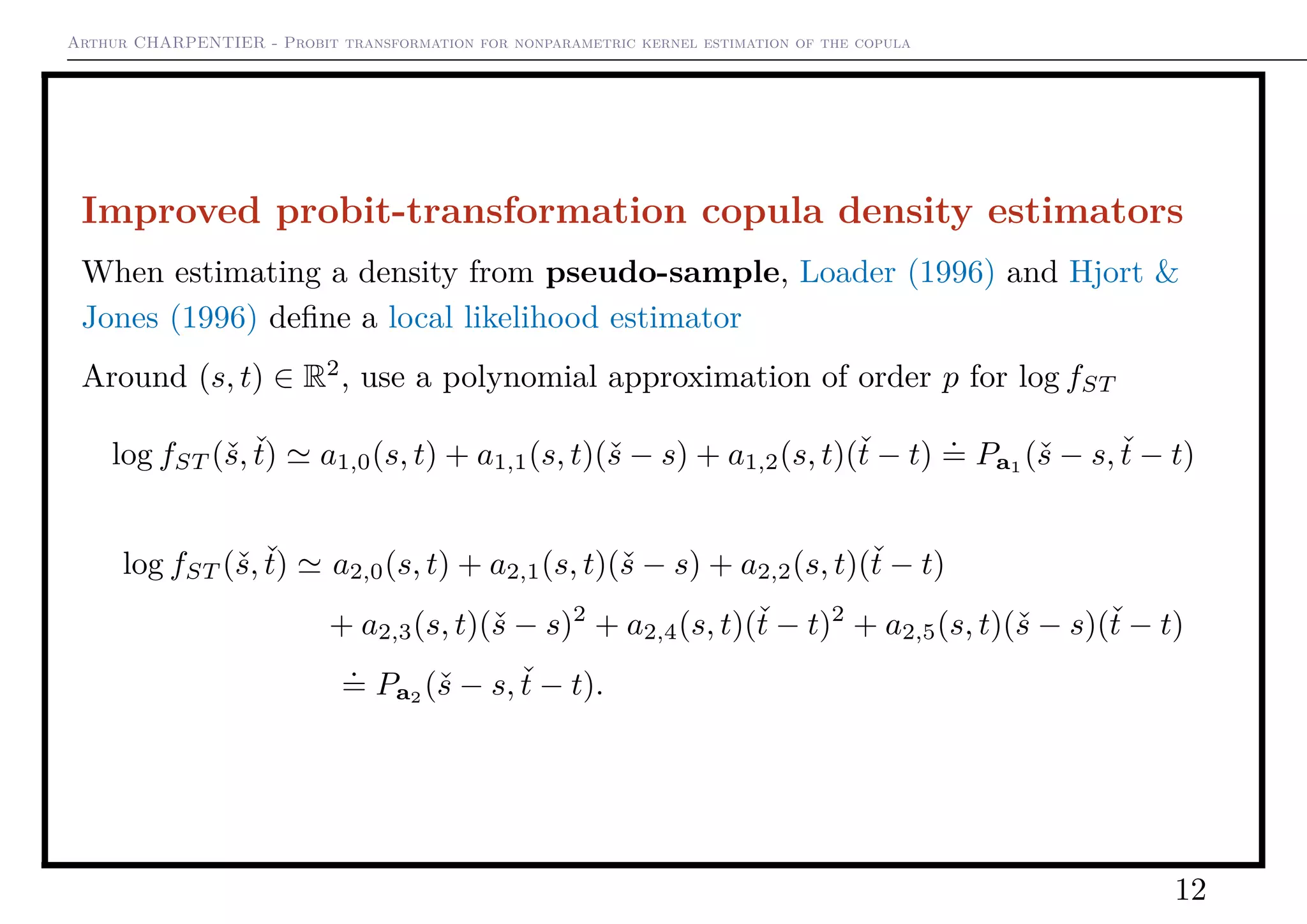
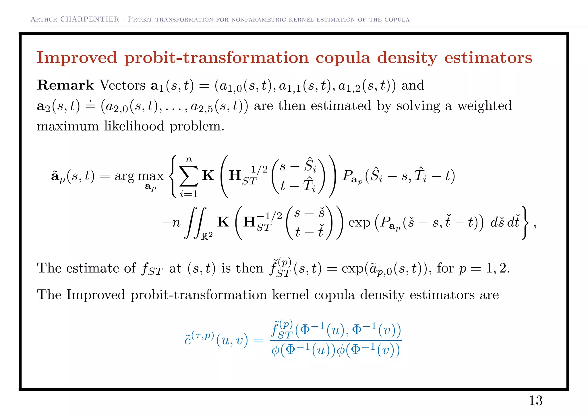
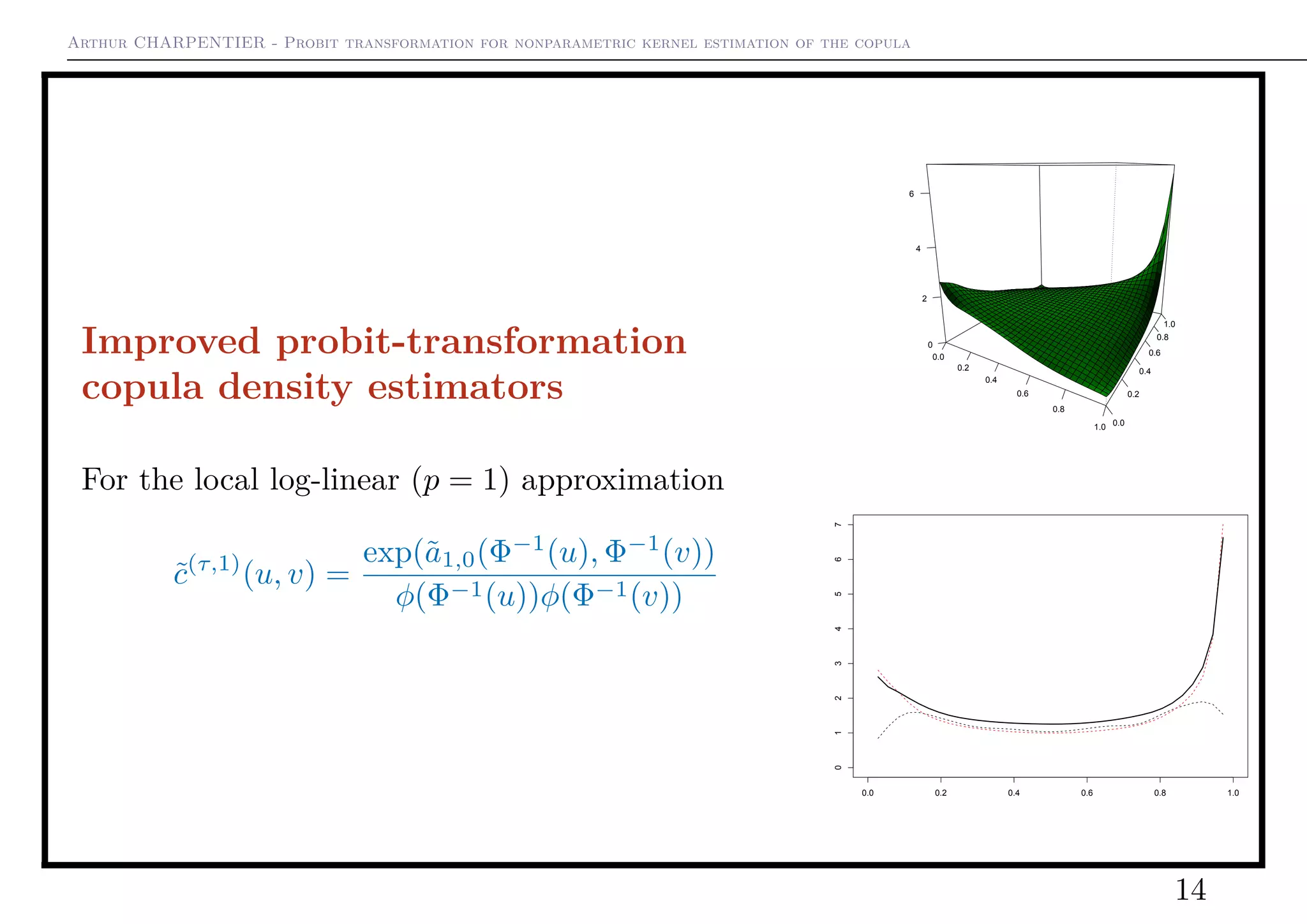
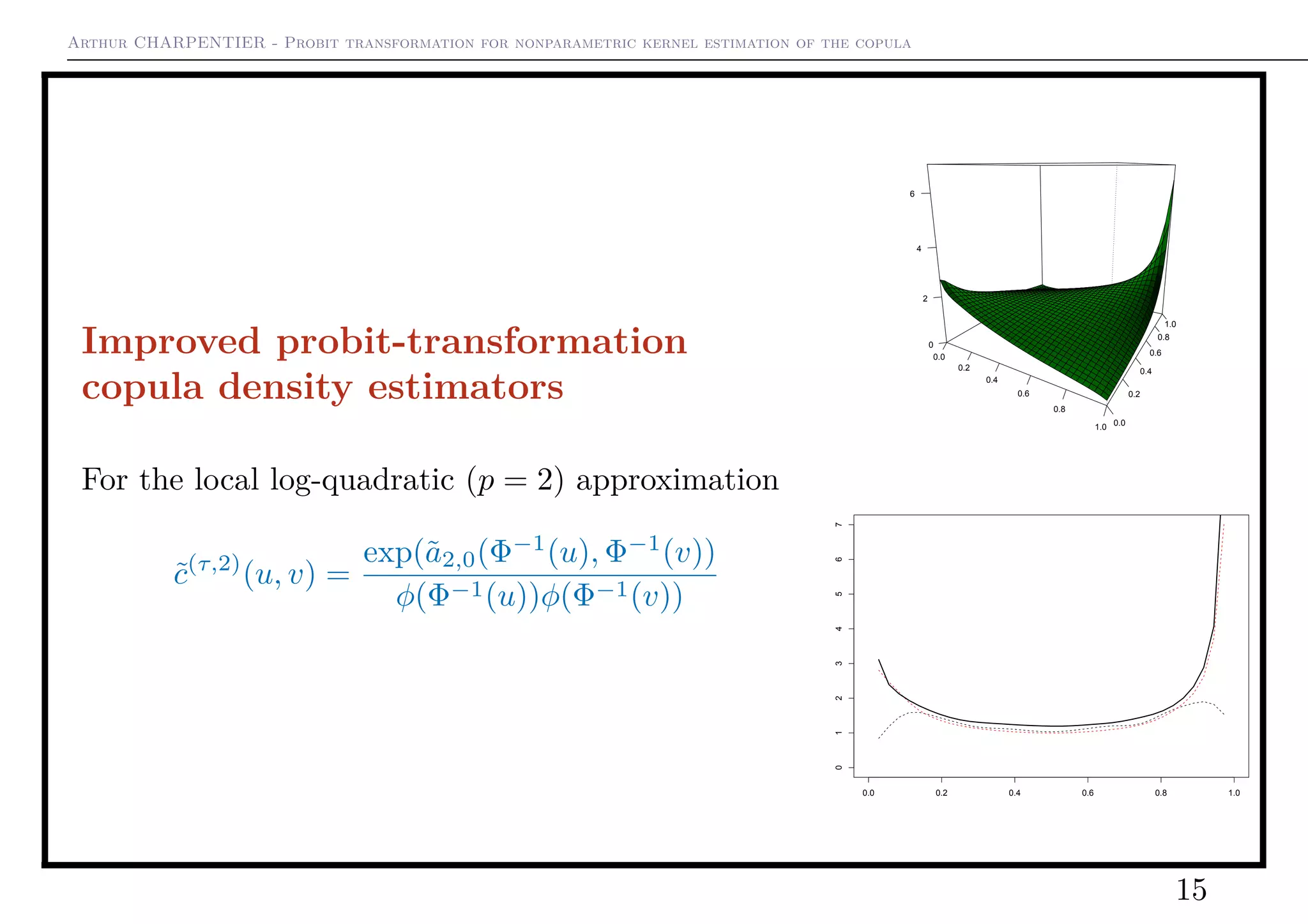
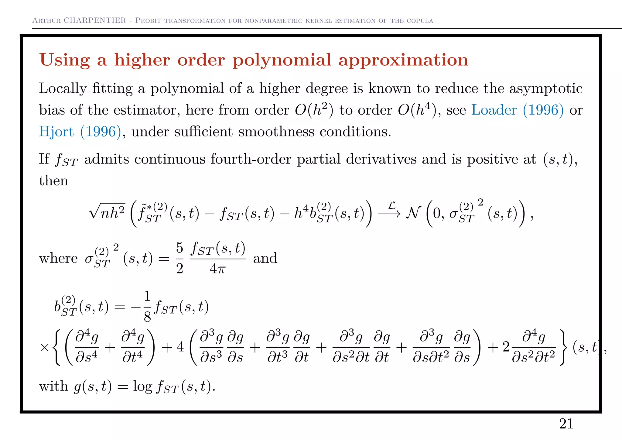
Using a higher order polynomial approximation
A4. The copula density c(u, v) = (∂2
C/∂u∂v)(u, v) admits continuous
fourth-order partial derivatives on the interior of the unit square [0, 1]2
.
Then
√
nh2 ˜c∗(τ,2)
(u, v) − c(u, v) − h4 b(2)
(u, v)
φ(Φ−1(u))φ(Φ−1(v))
L
−→ N 0, σ(2) 2
(u, v)
where σ(2) 2
(u, v) =
5
2
c(u, v)
4πφ(Φ−1(u))φ(Φ−1(v))
22](https://image.slidesharecdn.com/slides-cirm-2016-light-160208151543/75/slides-CIRM-copulas-extremes-and-actuarial-science-22-2048.jpg)
![Arthur CHARPENTIER - Probit transformation for nonparametric kernel estimation of the copula
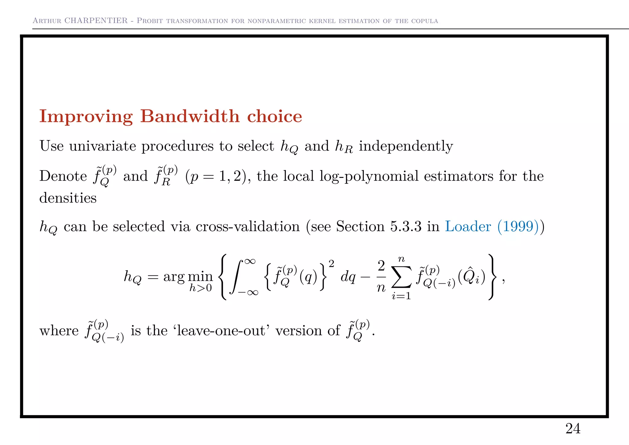
Improving Bandwidth choice
Consider the principal components decomposition of the (n × 2) matrix
[ˆS, ˆT ] = M.
Let W1 = (W11, W12)T
and W2 = (W21, W22)T
be the eigenvectors of MT
M. Set
Q
R
=
W11 W12
W21 W22
S
T
= W
S
T
which is only a linear reparametrization of R2
, so
an estimate of fST can be readily obtained from an
estimate of the density of (Q, R)
Since { ˆQi} and { ˆRi} are empirically uncorrelated,
consider a diagonal bandwidth matrix HQR =
diag(h2
Q, h2
R).
−4 −2 0 2 4
−3−2−1012
23](https://image.slidesharecdn.com/slides-cirm-2016-light-160208151543/75/slides-CIRM-copulas-extremes-and-actuarial-science-23-2048.jpg)

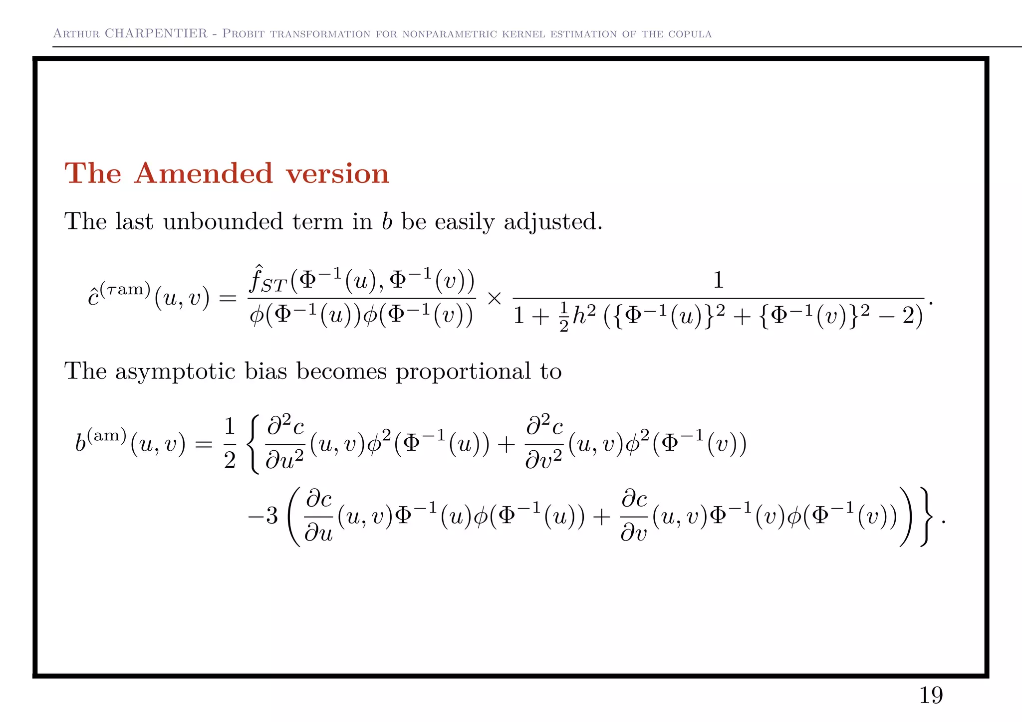
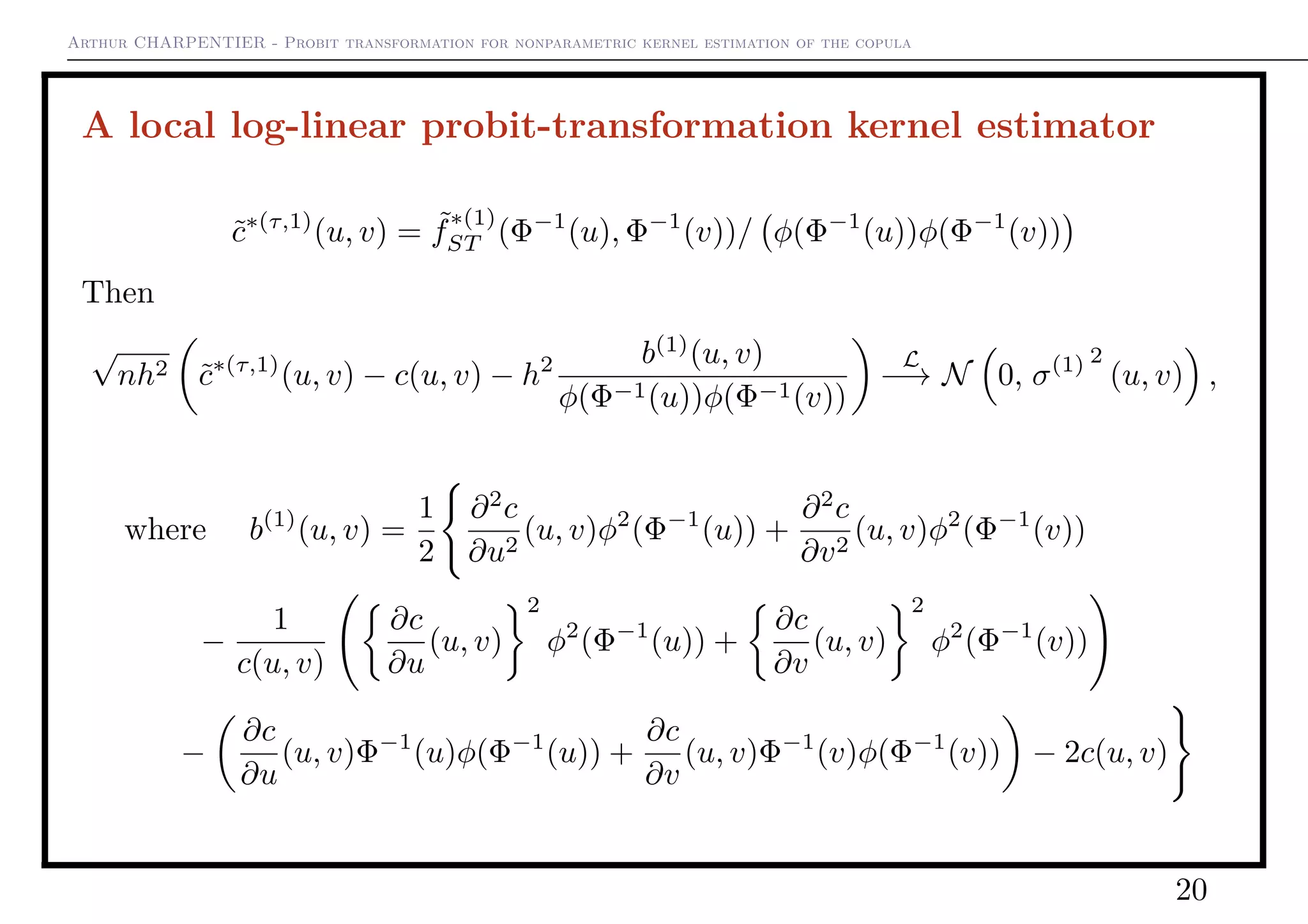
1) The document discusses probit transformation for nonparametric kernel estimation of copulas. It introduces a standard kernel estimator for copulas that is inconsistent on boundaries. 2) It then presents a "naive" probit transformation kernel copula density estimator that transforms data to standard normal using the probit function to address boundary issues. 3) It further improves upon this by introducing local log-linear and log-quadratic approximations for the transformed density, yielding two new estimators with better asymptotic properties.


![[DSC Europe 25] Dragana Ilic - AI for Big Data in Astronomy.pptx](https://cdn.slidesharecdn.com/ss_thumbnails/8palya86qaatvjhva1ms-2-dragana-ilic-ai-ilic-251208151906-652b819c-thumbnail.jpg?width=640&height=640&fit=bounds)


![[DSC Europe 25] Marija Vlajkovic & Andrea Radonjanin - Integration of AI tool...](https://cdn.slidesharecdn.com/ss_thumbnails/qf1jrglttoc3bm8s3aop-final-integration-of-ai-tools-251208151905-394f3a6a-thumbnail.jpg?width=640&height=640&fit=bounds)
![[DSC Europe 25] Andy Cotgreave - Nothing is new in analytics.pptx](https://cdn.slidesharecdn.com/ss_thumbnails/mba4vzcurvoh5lfrd5zw-6-251205194645-341bbbbe-thumbnail.jpg?width=640&height=640&fit=bounds)


![[DSC Europe 25] Vid Stimac - Policy Parsimony: Between Oversimplifying and Ov...](https://cdn.slidesharecdn.com/ss_thumbnails/eqlepagzqp2rhg3gbluh-dsc-stimac-251120-251205090438-059e7f54-thumbnail.jpg?width=640&height=640&fit=bounds)