Side 2019 #10

Arthur Charpentier, SIDE Summer School, July 2019
# 10 Times Series and Forecasting
Arthur Charpentier (Université du Québec à Montréal)
Machine Learning & Econometrics
SIDE Summer School - July 2019
@freakonometrics freakonometrics freakonometrics.hypotheses.org 1

Time Series
Time Series
A time series is a sequence of observations (yt) ordered in time.
Write yt = st + ut, with systematic part st (signal / trend) and ‘residual’ term ut
(ut) is supposed to be a strictly stationary time series
(st) might be a ‘linear’ trend, plus a seasonal cycle
Buys-Ballot (1847, Les changements périodiques de
température, dépendants de la nature du soleil et de la
lune, mis en rapport avec le pronostic du temps, déduits
d’observations néerlandaises de 1729 à 1846) - original
probably in Dutch.

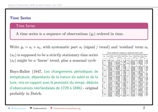
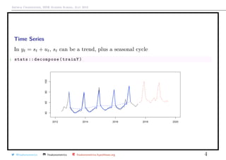
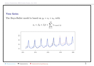
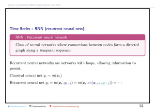
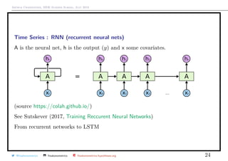
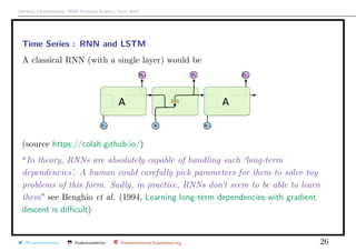
Time Series
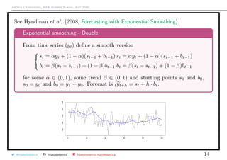
Consider the general prediction tyt+h = m(information available at time t)
1 hp <- read.csv("http:// freakonometrics .free.fr/ multiTimeline .csv",
skip =2)
2 T=86 -24
3 trainY <- ts(hp[1:T,2], frequency= 12, start= c(2012 , 6))
4 validY <- ts(hp[(T+1):nrow(hp) ,2], frequency= 12, start= c(2017 , 8))

Time Series
In yt = st + ut, st can be a trend, plus a seasonal cycle
1 stats :: decompose(trainY)

Time Series
The Buys-Ballot model is based on yt = st + ut, with
st = β0 + β1t +
12
h=1
γt mod 12

Time Series : Linear Trend ?
Various (machine learning) techniques can used, such as Laurinec (2017, Using
regression trees for forecasting double-seasonal time series with trend in R),
Bontempi et al. (2012, Machine Learning Strategies for Time Series Forecasting),
Dietterich (2002, Machine Learning for Sequential Data: A Review)

Time Series : Exponential Smoothing
“when Gardner (2005) appeared, many believed that exponential smoothing should
be disregarded because it was either a special case of ARIMA modeling or an ad
hoc procedure with no statistical rationale. As McKenzie (1985) observed, this
opinion was expressed in numerous references to my paper. Since 1985, the
special case argument has been turned on its head, and today we know that
exponential smoothing methods are optimal for a very general class of state-space
models that is in fact broader than the ARIMA class.”
from Hyndman et al. (2008, Forecasting with Exponential Smoothing)

Exponential smoothing - Simple
From time series (yt) deﬁne a smooth version
st = α · yt + (1 − α) · st−1 = st−1 + α · (yt − st−1)
for some α ∈ (0, 1) and starting point s0 = y1 Forecast is tyt+h = st
It is called exponential smoothing since
st = αyt + (1 − α)st−1
= αyt + α(1 − α)yt−1 + (1 − α)2
st−2
= α yt + (1 − α)yt−1 + (1 − α)2
yt−2 + (1 − α)3
yt−3 + · · · + (1 − α)t−1
y1 + (1 − α)t
y
corresponding to exponentially weighted moving average
Need to adapt cross-validation techniques,

Optimal α ? α ∈ argmin
T
t=2
2(yt − t−1yt) (leave-one-out strategy)

T
t=2

See Hyndman et al. (2008, Forecasting with Exponential Smoothing)
Exponential smoothing - Double
st = αyt + (1 − α)(st−1 + bt−1)
bt = β(st − st−1) + (1 − β)bt−1
st = αyt + (1 − α)(st−1 + bt−1)
bt = β(st − st−1) + (1 − β)bt−1
for some α ∈ (0, 1), some trend β ∈ (0, 1) and starting points s0 and b0,
s0 = y0 and b0 = y1 − y0. Forecast is tyt+h = st + h · bt.

st = αyt + (1 − α)(st−1 + bt−1)
bt = β(st − st−1) + (1 − β)bt−1
st = αyt + (1 − α)(st−1 + bt−1)
bt = β(st − st−1) + (1 − β)bt−1

Exponential smoothing - Seasonal with lag L (Holt-Winters)



st = α
xt
ct−L
+ (1 − α)(st−1 + bt−1)
bt = β(st − st−1) + (1 − β)bt−1
ct = γ
yt
st
+ (1 − γ)ct−L
for some α ∈ (0, 1), some trend β ∈ (0, 1), some seasonal change smoothing
factor, γ ∈ (0, 1) and starting points s0 = y0. Forecast is tyt+h = (st +
hbt)ct−L+1+(h−1) mod L.
See stats::HoltWinters()

1 hw_fit <- stats :: HoltWinters (trainY)
2 library(forecast)
3 plot(forecast(hw_fit , h=30))
4 lines(validY ,col="red")

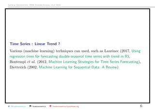
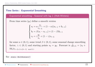
Time Series : State Space Models
See De Livera, Hyndman & Snyder (2011, Forecasting Time Series With Complex
Seasonal Patterns Using Exponential Smoothing),based on Box-Cox transformation
on yt: y
(λ)
t =
yλ
t − 1
λ
if λ = 0 (otherwise log yt)
See forecast::tbats
1 library(forecast)
2 forecast :: tbats(trainY)$lambda
3 [1] 0.2775889

1 library(forecast)
2 tbats_fit <- tbats(trainY)
3 plot(forecast(tbats_fit , h=30))
4 lines(validY , col="red")

Exponential smoothing state space model with Box-Cox transformation, ARMA
errors, Trend and Seasonal components
y
(λ)
t = t−1 + φbt−1 +
T
i=1
s
(i)
t−mi
+ dt where
• ( t) is some local level, t = t−1 + φbt−1 + αdt
• (bt) is some trend with damping, bt = φbt−1 + αdt
• (dt) is some ARMA process for the stationary component
dt =
p
i=1
ϕidt−i + t +
q
j=1
θj t−j
• (s
(i)
t ) is the i-th seasonal component

Let xt denote state variables (e.g. level,
slope, seasonal).
Classical statistical approach: compute
likelihood from errors ε1, · · · , εT
see forecast::ets
Innovations state space models
Let xt = (st, bt, ct) and suppose εt i.i.d. N(0, σ2
)
State equation : xt = f(xt−1) + g(xt−1)εt
Observation equation : yt = µt + et = h(xt−1) + σ(xt−1)εt
Inference based on log L = n log
T
t=1
ε2
t
σ(xt−1)
+ 2
T
t=1
log |σ(xt−1)|
One can use time series cross-validation, valued on a rolling forecast origin

1 library(forecast)
2 ets_fit <- forecast ::ets(trainY)
3 plot(forecast(ets_fit , h=30))

Time Series : Automatic ARIMA
Consider a general seasonal ARIMA process,
Φs(Ls
)Φ(L)(1 − L)d
(1 − Ls
)ds
yt = c + Θs(Ls
)Θ(L)εt
See forecast::autoarima(, include.drift=TRUE) , “Automatic algorithms will become
more general - handling a wide variety of time series” (Rob Hyndman)

Time Series : RNN (recurrent neural nets)
RNN : Recurrent neural network
Class of neural networks where connections between nodes form a directed
graph along a temporal sequence.
Recurrent neural networks are networks with loops, allowing information to
persist.
Classical neural net yi = m(xi)
Recurrent neural net yt = m(xt, yt−1) = m(xt, m(xt−1, yt−2)) = · · ·

Time Series : RNN (recurrent neural nets)
A is the neural net, h is the output (y) and x some covariates.
(source https://colah.github.io/)
See Sutskever (2017, Training Reccurent Neural Networks)
From recurrent networks to LSTM

Time Series : RNN and LTSM
(source Greﬀ et al. (2017, LSTM: A Search Space Odyssey))
see Hochreiter & Schmidhuber (1997, Long Short-Term Memory)

Time Series : RNN and LSTM
A classical RNN (with a single layer) would be
(source https://colah.github.io/)
“In theory, RNNs are absolutely capable of handling such ‘long-term
dependencies’. A human could carefully pick parameters for them to solve toy
problems of this form. Sadly, in practice, RNNs don’t seem to be able to learn
them” see Benghio et al. (1994, Learning long-term dependencies with gradient
descent is diﬃcult)

Time Series : RNN and LSTM
“RNNs can keep track of arbitrary long-term dependencies in the input
sequences.The problem of “vanilla RNNs” is computational (or practical) in
nature: when training a vanilla RNN using back-propagation, the gradients which
are back-propagated can “vanish” (that is, they can tend to zero) “explode” (that
is, they can tend to inﬁnity), because of the computations involved in the process”
(from wikipedia)

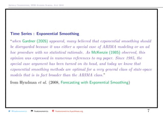
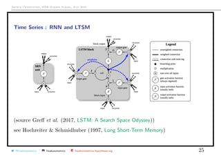
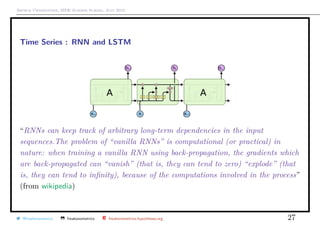
Time Series : LSTM
C is the long-term state
H is the short-term state
forget gate: ft = sigmoid(Af [ht−1, xt] + bf )
input gate: it = sigmoid(Ai[ht−1, xt] + bi)
new memory cell: ˜ct = tanh(Ac[ht−1, xt] + bc)

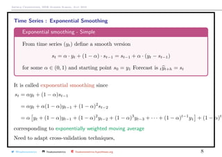
Time Series : LSTM
ﬁnal memory cell: ct = ft · ct−1 + it · ˜ct
output gate: ot = sigmoid(Ao[ht−1, xt] + bo)
ht = ot · tanh(ct)

Elicitable Measures & Forecasting
“elicitable” means “being a minimizer of a suitable expected score”, see Gneiting
(2011) Making and evaluating point forecasts.
Elicitable function
T is an elicatable function if there exits a scoring function S : R×R → [0, ∞)
T(Y ) = argmin
x∈R R
S(x, y)dF(y) = argmin
x∈R
E S(x, Y ) where Y ∼ F
Example: mean, T(Y ) = E[Y ] is elicited by S(x, y) = x − y 2
2
Example: median, T(Y ) = median[Y ] is elicited by S(x, y) = x − y 1
Example: quantile, T(Y ) = QY (τ) is elicited by
S(x, y) = τ(y − x)+ + (1 − τ)(y − x)−
Example: expectile, T(Y ) = EY (τ) is elicited by
S(x, y) = τ(y − x)2
+ + (1 − τ)(y − x)2
−

Forecasts and Predictions
Mathematical statistics is based on inference and testing, using probabilistic
properties.
If we can reproduce past observations, it is supposed to proved good predictions.
Why not consider a collection of scenarios likely to occur on a given time horizon
(drawing fro, a (predictive) probability distribution)
The closer forecast yt is to observed yt, the better the model, either according to
1-norm - with |yt − yt| - or to the 2-norm - with (yt − yt)2
.
If this is an interesting information about central tendency, it cannot be used to
anticipate extremal events.

Forecasts and Predictions
More formally, we try to compare two very diﬀerent objects : a function (the
predictive probability distribution) and a real value number (the observed value).
Natural idea : introduce a score, as in Good (1952, Rational Decisions) or Winkler
(1969, Scoring Rules and the Evaluation of Probability Assessors), used in
meteorology by Murphy & Winkler (1987, A General Framework for Forecast
Veriﬁcation).
Let F denote the predictive distribution, expressing the uncertainty attributed to
future values, conditional on the available information.

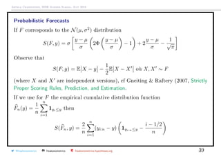
Probabilistic Forecasts
Notion of probabilistic forecasts, Gneiting & Raftery (2007 Strictly Proper Scoring
Rules, Prediction, and Estimation).
In a general setting, we want to predict value taken by random variable Y .
Let F denote a cumulative distribution function.
Let A denote the information available when forecast is made.
F is the ideal forecast for Y given A if the law of Y |A has distribution F.
Suppose F continuous. Set ZF = F(Y ), the probability integral transform of Y .
F is probabilistically calibrated if ZF ∼ U([0, 1])
F is marginally calibrated if E[F(y)] = P[Y ≤ y] for any y ∈ R.

Observe that for a ideal forecast, F(y) = P[Y ≤ y|A], then
• E[F(y)] = E[P[Y ≤ y|A]] = P[Y ≤ y]
This forecast is est marginally calibrated
• P[ZF ≤ z] = E[P[ZF ≤ z|A]] = z
This forecast is probabilistically calibrated
Suppose µ ∼ N(0, 1). And that ideal forecast is Y |µ ∼ N(µ, 1).
E.g. if Yt ∼ N(0, 1) and Yt+1 = yt + εt ∼ N(yt, 1).
One can consider F = N(0, 2) as na¨ıve forecast. This distribution is marginally
calibrated, probabilistically calibrated and ideal.
One can consider F a mixture N(µ, 2) and N(µ ± 1, 2) where ”±1” means +1 or
−1 probability 1/2, hesitating forecast. This distribution is probabilistically
calibrated, but not marginally calibrated.

Indeed P[F(Y ) ≤ u] = u,
P[F(Y ) ≤ u] =
P[Φ(Y ) ≤ u] + P[Φ(Y + 1) ≤ u]
2
+
P[Φ(Y ) ≤ u] + P[Φ(Y − 1) ≤ u]
2
One can consider F = N(−µ, 1). This distribution is marginally calibrated, but
not probabilistically calibrated.
In practice, we have a sequence (Yt, Ft) of pairs, (Y , F ).
The set of forecasts F is said to be performant if for all t, predictive distributions
Ft are precise (sharpness) and well-calibrated.
Precision is related to the concentration of the predictive density around a
central value (uncertainty degree).
Calibration is related to the coherence between predictive distribution Ft and
observations yt.

Calibration is poor if 80%-conﬁdence intervals (implied from predictive
distributions, i.e. F−1
t (α), F−1
t (1 − α) ) do not contain yt’s about 8 times out of
10.
To test marginal calibration, compare the empirical cumulative distribution
function
G(y) = lim
n→∞
1
n
1Yt≤y
and the average of predictive distributios
F(y) = lim
n→∞
1
n
n
t=1
Ft(y)
To test probabilistic calibration, test if sample {Ft(Yt)} has a uniform
distribution - PIT approach, see Dawid (1984, Present Position and Potential
Developments: The Prequential Approach).

One can also consider a score S(F, y) for all distribution F and all observation y.
The score is said to be proper if
∀F, G, E[S(G, Y )] ≤ E[S(F, Y )] where Y ∼ G.
In practice, this expected value is approximated using
1
n
n
t=1
S(Ft, Yt)
One classical rule is the logarithmic score S(F, y) = − log[F (y)] if F is (abs.)
continuous.
Another classical rule is the continuous ranked probability score (CRPS, see
Hersbach (2000, Decomposition of the Continuous Ranked Probability Score for
Ensemble Prediction Systems))
S(F, y) =
+∞
−∞
(F(x) − 1x≥y)2
dx =
y
−∞
F(x)2
+
+∞
y
(F(x) − 1)2
dx

with empirical version
S =
1
n
n
t=1
S(Ft, yt) =
1
n
n
t=1
+∞
−∞
(Ft(x) − 1x≥yt
)2
dx
studied in Murphy (1970, The ranked probability score and the probability score: a
comparison).
This rule is proper since
E[S(F, Y )] =
∞
−∞
E F(x) − 1x≥Y
2
dx
=
∞
−∞
[F(x) − G(x)]2
+ G(x)[1 − G(x)]
2
dx
is minimal when F = G.

If F corresponds to the N(µ, σ2
) distribution
S(F, y) = σ
y − µ
σ
2Φ
y − µ
σ
− 1 + 2
y − µ
σ
−
1
√
π
Observe that
S(F, y) = E X − y −
1
2
E X − X o`u X, X ∼ F
(where X and X are independent versions), cf Gneiting & Raftery (2007, Strictly
Proper Scoring Rules, Prediction, and Estimation.
If we use for F the empirical cumulative distribution function
Fn(y) =
1
n
n
i=1
1yi≤y then
S(Fn, y) =
2
n
n
i=1
(yi:n − y) 1yi:n≤y −
i − 1/2
n

Consider a Gaussian AR(p) time series,
Yt = c + ϕ1Yt−1 + · · · + ϕpYt−p + εt, with εt ∼ N(0, σ2
)
then forecast with horizon 1 yields
Ft ∼ N(t−1Yt, σ2
)
where t−1Yt = c + ϕ1Yt−1 + · · · + ϕpYt−p.

Suppose that Y can be explained by covariates x = (x1, · · · , xm). Consider some
kernel based conditional density estimation
p(y|x) =
p(y, x)
p(x)
=
n
i=1 Kh(y − yi)Kh(x − xi)
n
i=1 Kh(x − xi)
In the case of a linear model, there exists θ such that p(y|x) = p(y|θT
x), and
p(y|θT
x = s) =
n
i=1 Kh(y − yi)Kh(s − θT
xi)
n
i=1 Kh(s − θT
xi)
Parameter θ can be estimated using a proxy of the log-likelihood
θ = argmax
n
i=1
log p(yi|θT
xi)

Time Series : Stacking
See Clemen (1989, Combining forecasts: A review and annotated bibliography)
See opera::oracle(Y = Y, experts = X, loss.type =’square’, model =’convex’)
(on Online Prediction by Expert Aggregation)

Natural Language Processing & Probabilistic Language Models
Idea : P[today is Wednesday] > P[today Wednesday is]
Idea : P[today is Wednesday] > P[today is Wendy]
E.g. try to predict the missing word I grew up in France, I speak ﬂuent

Natural Language Processing & Probabilistic Language Models
Use of the chain rule
P[A1, A2, · · · , An] =
n
i=1
P[Ai|A1, A2, · · · , Ai−1]
P(the wine is so good)
= P(the) · P(wine|the) · P(is|the wine) · P(so|the wine is) · P(good|the wine is so)
Markov assumption & k-gram model
P[A1, A2, · · · , An] ∼
n
i=1
P[Ai|Ai−k, · · · , Ai−1]

Side 2019 #10

More Related Content

What's hot

Similar to Side 2019 #10

More from Arthur Charpentier

Recently uploaded

Side 2019 #10