Downloaded 16 times

![Arthur CHARPENTIER - Rennes Risk Workshop - April, 2015
Aumann & Serrano Riskiness
– Given X, the index of risk R(X) is defined to be the unique positive solution
(if exists) of E[exp(−X/R(X))] = 1
– Index of Riskiness x → R :
R such that exp −
x
R
U(x)
dF(x) = 1
where U is CARA.
4](https://image.slidesharecdn.com/slides-risk-rennes-150401072238-conversion-gate01/75/Slides-risk-rennes-4-2048.jpg)
![Arthur CHARPENTIER - Rennes Risk Workshop - April, 2015
Local utility
– Decision maker ranks random vectors X with law invariant functional
Φ(X) = Φ(FX), with FX the cdf of X.
– Local utility x → U(x; F) is the Fréchet derivative of Φ at F :
Φ(F ) − Φ(F) − U(x; F)[dF (x) − dF(x)] → 0
– If Φ is expected utility, local and global utilities coincide
– If Φ is the Quiggin-Yaari functional Φ(X) = φ(t)F−1
X (t)dt, then local
utility is U(x; F) =
x
−∞
φ(F(z))dz
– If Φ is the Aumann-Serrano index of riskiness, the local utility
cst[1 − exp(−αx)] is CARA
5](https://image.slidesharecdn.com/slides-risk-rennes-150401072238-conversion-gate01/75/Slides-risk-rennes-5-2048.jpg)
![Arthur CHARPENTIER - Rennes Risk Workshop - April, 2015
Rothschild-Stiglitz mean preserving increase in risk
One of the most commonly used stochastic orderings to compare risky prospects
is the mean preserving increase in risk (MPIR or concave ordering). Let X and Y
be two prospects.
Definition :
Y MP IR X if E[u(X)] ≥ E[u(Y )] for all concave utility u.
Characterization :
∗ Y
L
= X + Z with E[Z|X] = 0 (where “
L
=” denotes equality in distribution).
6](https://image.slidesharecdn.com/slides-risk-rennes-150401072238-conversion-gate01/75/Slides-risk-rennes-6-2048.jpg)
![Arthur CHARPENTIER - Rennes Risk Workshop - April, 2015
Local utility and MPIR
– Aversion to MPIR is equivalent to concavity of local utility (Machina 1982 for
the univariate result)
– Still holds for multivariate risks :
– Φ is MPIR averse (Schur concave) if Φ(Y ) ≤ Φ(X) when Y is an MPIR of
X.
– Equivalent to concavity of U(x; F) in x for all distributions F
Proof : Φ Schur concave iff Φ decreasing along all martingales Xt
Φ(Xt+dt) − Φ(Xt) = E [U(Xt+dt; FXt ) − U(Xt; FXt )]
= E Tr D2
U(Xt; FXt )σT
t σt Itô
≤ 0 iff U(x; F) concave
7](https://image.slidesharecdn.com/slides-risk-rennes-150401072238-conversion-gate01/75/Slides-risk-rennes-7-2048.jpg)


![Arthur CHARPENTIER - Rennes Risk Workshop - April, 2015
Local utility and attitude to mean preserving dispersion
increase (Quiggin’s monotone MPIR)
– Φ is MMPIR averse if and only if
E
U (X; FX)
E[U (X; FX)]
1{X > x} ≤ E [1{X > x}]
– Example : Quiggin-Yaari functional
Φ(X) = φ(t)F−1
X (t)dt
with local utility is
U(x; F) =
x
−∞
φ(FX(z))dz
is MMPIR averse iff density φ(u) is stochastically dominated by the uniform
(called pessimism by Quiggin)
10](https://image.slidesharecdn.com/slides-risk-rennes-150401072238-conversion-gate01/75/Slides-risk-rennes-10-2048.jpg)


![Arthur CHARPENTIER - Rennes Risk Workshop - April, 2015
Revisiting comonotonicity
– X and Y are comonotonic if there exists Z such that X = TX(Z) and
Y = TY (Z), TX, TY increasing functions.
– Example :
– If X(ωi) = xi and Y (ωi) = yi, i = 1 . . . , n, with x1 ≤ . . . ≤ xn and
y1 ≤ . . . ≤ yn, then X and Y are comonotonic.
– By the simple rearrangement inequality,
i=1,...,n
xiyi = max
i=1,...,n
xiyσ(i) : σ permutation
.
– General characterization : X and Y are comonotonic iff
E[XY ] = sup E[X ˜Y ] : ˜Y
L
= Y .
14](https://image.slidesharecdn.com/slides-risk-rennes-150401072238-conversion-gate01/75/Slides-risk-rennes-14-2048.jpg)
![Arthur CHARPENTIER - Rennes Risk Workshop - April, 2015
Revisiting the quantile function
The quantile function of a prospect X is the generalized inverse of the cumulative
distribution function :
u → QX(u) = inf{x : P(X ≤ x) ≥ u}
Equivalent characterizations :
– The quantile function QX of a prospect X is an increasing rearrangement of X,
– The quantile QX(U) of X is the version of X which is comonotonic with the
uniform random variable U on [0, 1].
– QX is the only l.s.c. increasing function such that
E[QX(U)U] = sup{E[ ˜XU]; ˜X
L
= X}.
15](https://image.slidesharecdn.com/slides-risk-rennes-150401072238-conversion-gate01/75/Slides-risk-rennes-15-2048.jpg)
![Arthur CHARPENTIER - Rennes Risk Workshop - April, 2015
Multivariate µ-quantiles and µ-comonotonicity, (Galichon and
Henry, JET 2012)
– The univariate quantile function of a random variable X is the only l.s.c.
increasing function such that
E[QX(U)U] = sup{E[ ˜XU]; ˜X
L
= X}.
– Similarly, the µ-quantile QX is the essentially unique gradient of a l.s.c.
convex function (Brenier, CPAM 1991),
E[ QX(U), U ] = sup{E[ ˜X, U ]; ˜X
L
= X}, for some U
L
= µ.
– X and Y are µ-comonotonic if for some U
L
= µ,
X = QX(U) and Y = QY (U),
namely if X and Y can be simultaneously rearranged relative to a reference
distribution µ.
16](https://image.slidesharecdn.com/slides-risk-rennes-150401072238-conversion-gate01/75/Slides-risk-rennes-16-2048.jpg)
![Arthur CHARPENTIER - Rennes Risk Workshop - April, 2015
Example : Gaussian prospects
Suppose the baseline U is standard normal,
– X ∼ N(0, ΣX), hence X = Σ
1/2
X OXU, with OX orthogonal,
– Y ∼ N(0, ΣY ), hence Y = Σ
1/2
Y OY U, with OY orthogonal,
E[ ˜X, U ] is minimized for ˜X = Σ
1/2
X U, so when OX is the identity. Hence the
generalized quantile of X relative to U is
QX(U) = Σ
1/2
X U.
X and Y are N(0, I)-comonotonic if OX = OY (they have the same orientation).
The correlation is
E[XY T
] = Σ
1/2
X OXOT
Y Σ
1/2
Y = Σ
1/2
X Σ
1/2
Y .
17](https://image.slidesharecdn.com/slides-risk-rennes-150401072238-conversion-gate01/75/Slides-risk-rennes-17-2048.jpg)
![Arthur CHARPENTIER - Rennes Risk Workshop - April, 2015
Computation of generalized quantiles
The optimal transportation map between µ on [0, 1]d
and the empirical
distribution relative to (X1, . . . , Xn) satisfies
– ˆQX(U) ∈ {X1, . . . , Xn}
– µ( ˆQ−1
X ({Xk})) = 1/n, for each k = 1, . . . , n
– ˆQX is the gradient of a convex function V : Rd
→ R.
The solution for the “potential” V is
V (u) = max
k
{ u, Xk − wk},
where w = (w1, . . . , wn) minimizes the convex function
w → V (u)dµ(u) +
n
k=1
wk/n.
18](https://image.slidesharecdn.com/slides-risk-rennes-150401072238-conversion-gate01/75/Slides-risk-rennes-18-2048.jpg)
![Arthur CHARPENTIER - Rennes Risk Workshop - April, 2015
Multivariate Quiggin-Yaari functional and risk attitude
– Given a baseline U ∼ µ, decision maker evaluates risks with the functional
Φ(X) = E[QX(U) · φ(U)]
(Equivalent to monotonicity relative to stochastic dominance and comonotonic
additivity of Φ - Galichon and Henry JET 2012)
– Aversion to MPIR is equivalent to Φ(U) = −U
– Aversion to MMPIR is equivalent to Φ(X) ≤ Φ(E[X]) (obtains immediately
from the comonotonicity characterization of Bickel-Lehmann dispersion)
22](https://image.slidesharecdn.com/slides-risk-rennes-150401072238-conversion-gate01/75/Slides-risk-rennes-22-2048.jpg)

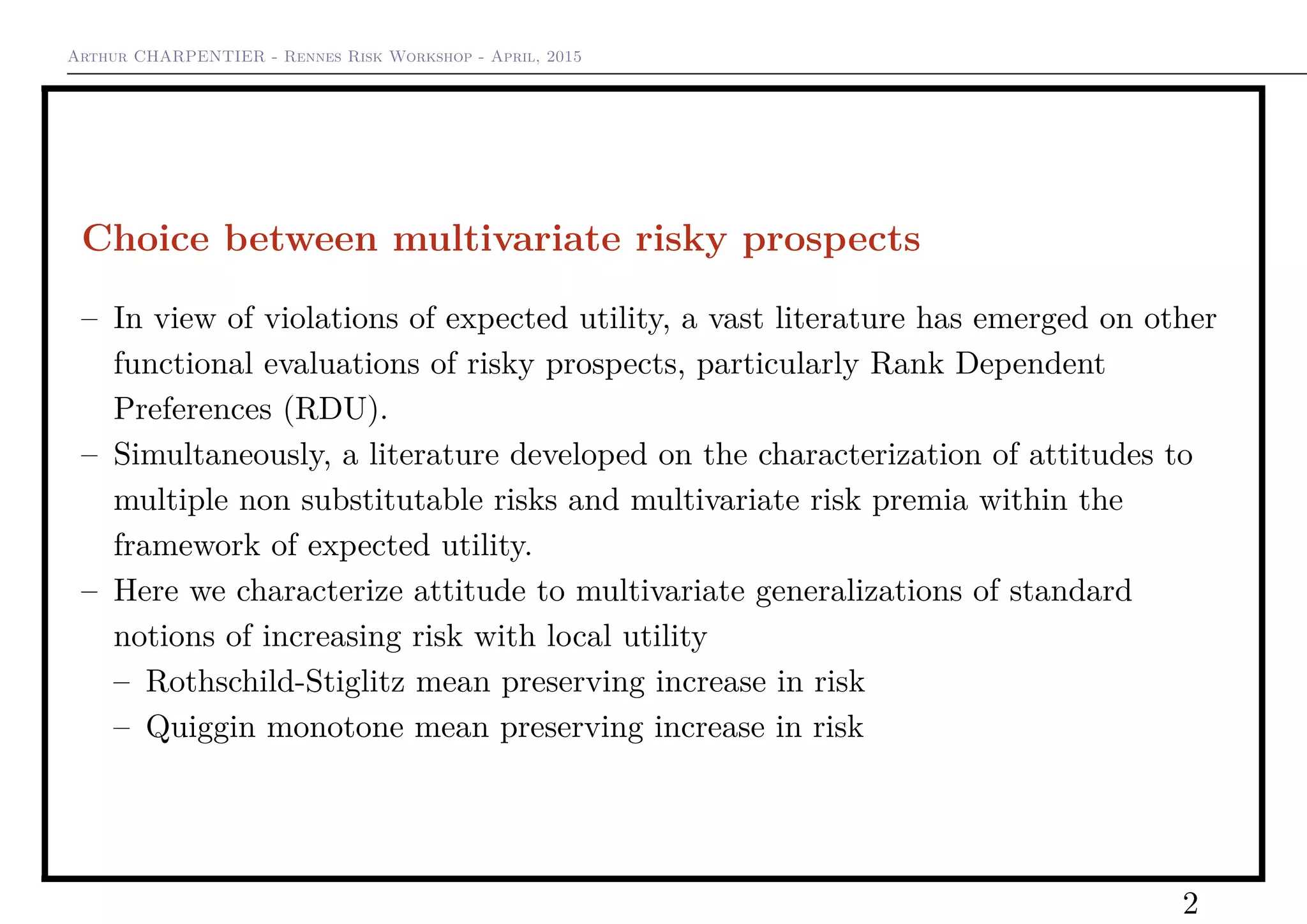
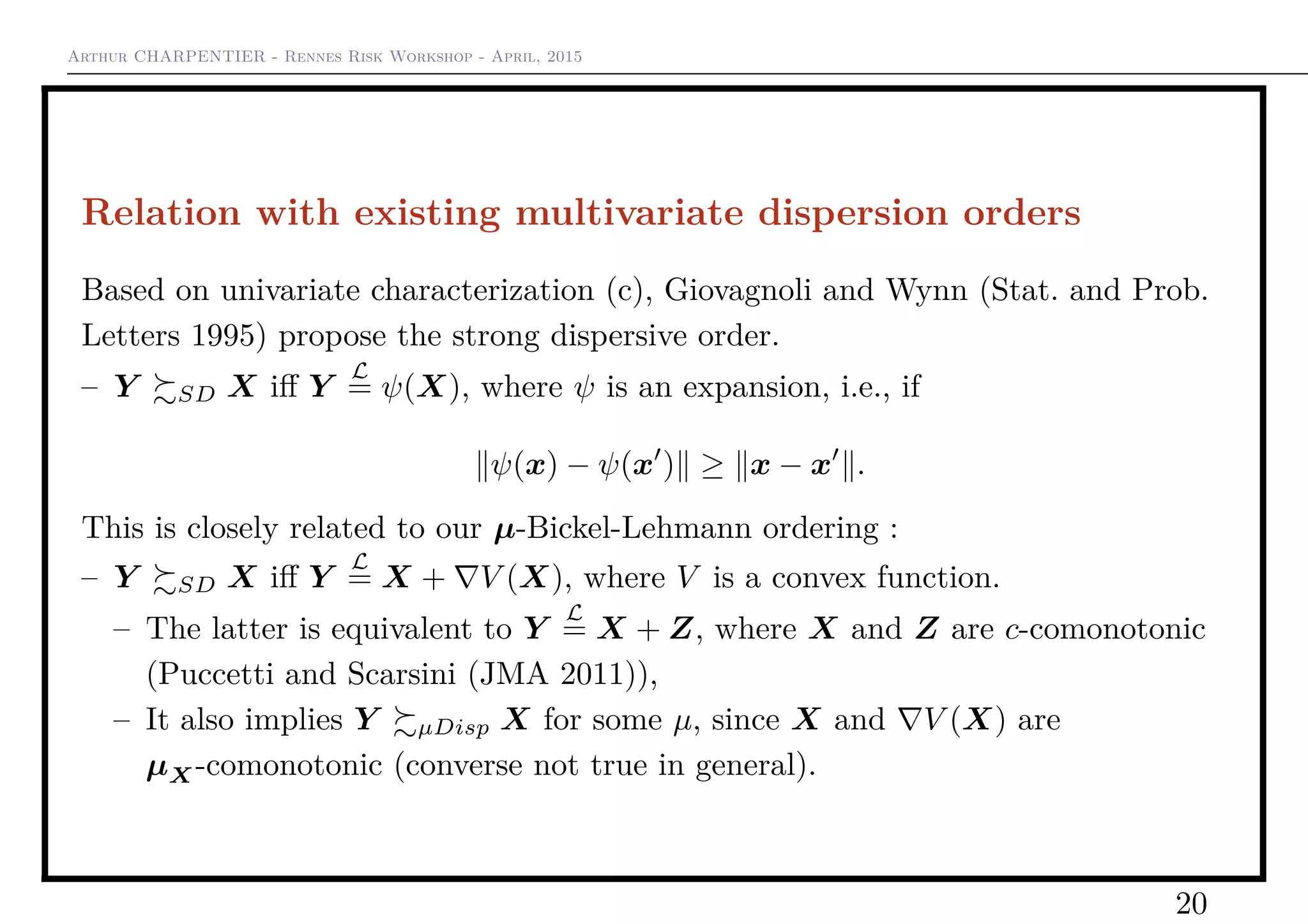
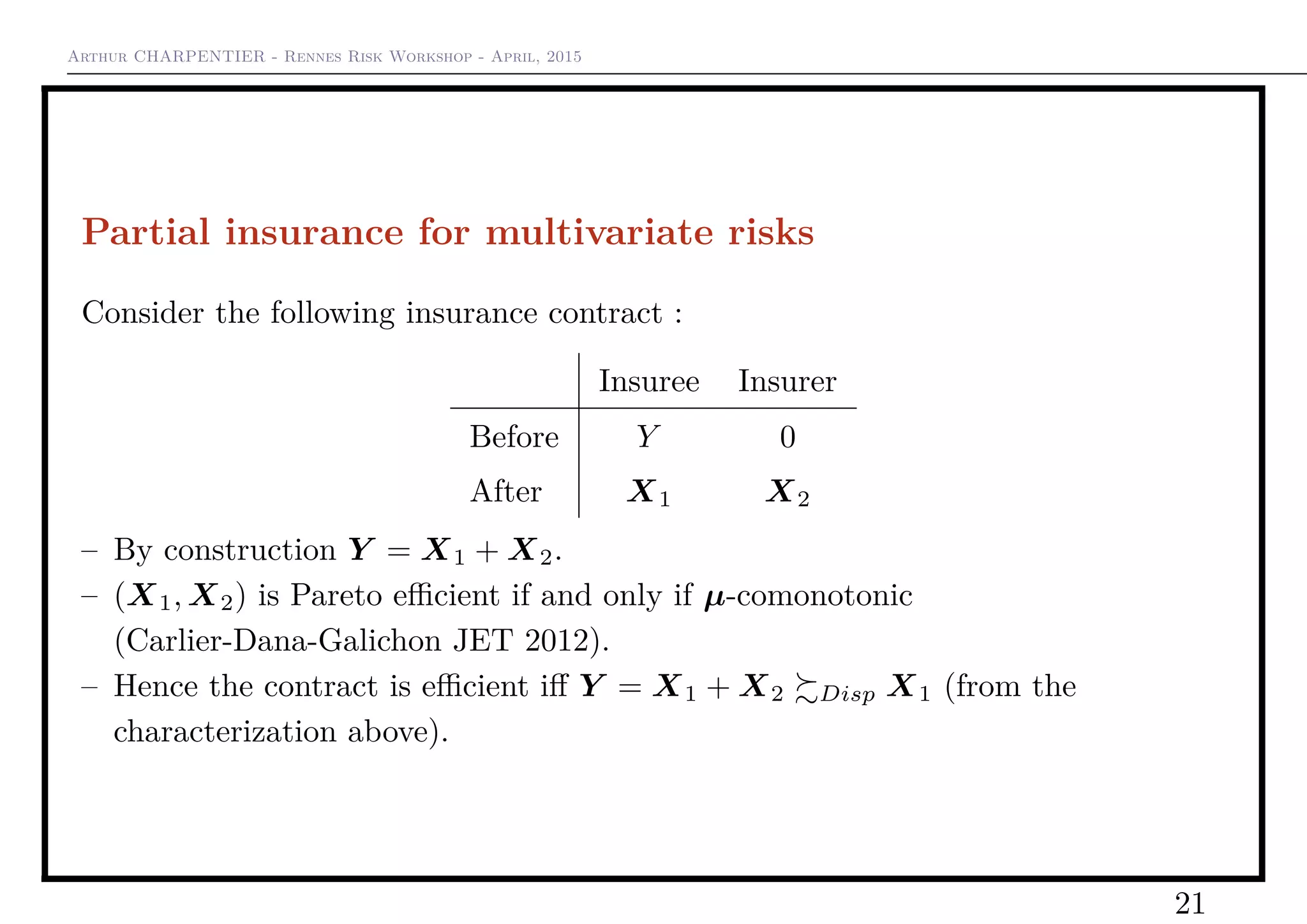
This document summarizes Arthur Charpentier's presentation at the Rennes Risk Workshop in April 2015. It discusses extending concepts of risk from univariate to multivariate prospects, including characterizing attitudes to multivariate notions of increasing risk like the Rothschild-Stiglitz mean preserving increase in risk and Quiggin's monotone mean preserving increase in risk. It also generalizes the Bickel-Lehmann dispersion order to multivariate risks and examines its implications for risk sharing.


