This document discusses kernel-based estimation methods for inequality indices and risk measures. It begins with an overview of stochastic dominance and related indices like first-order, convex, and second-order stochastic dominance. It then discusses nonparametric estimation of densities and copula densities using kernel methods. Specifically, it proposes using beta kernels and transformed kernels to improve estimation at the boundaries. The document explores combining these approaches and using mixtures of distributions like beta distributions within the kernels. It concludes by discussing applications to heavy-tailed distributions.

1. Arthur CHARPENTIER - Rennes, SMART Workshop, 2014
Kernel Based Estimation
of Inequality Indices and Risk Measures
Arthur Charpentier
arthur.charpentier@univ-rennes1.fr
http://freakonometrics.hypotheses.org/
based on joint work with E. Flachaire
initiated by some joint work with
A. Oulidi, J.D. Fermanian, O. Scaillet, G. Geenens and D. Paindaveine
(Université de Rennes 1, 2015)
1

2. Arthur CHARPENTIER - Rennes, SMART Workshop, 2014
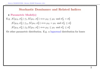
Stochastic Dominance and Related Indices
• First Order Stochastic Dominance (cf standard stochastic order, st)
X 1 Y ⇐⇒ FX(t) ≥ FY (t), ∀t ⇐⇒ VaRX(u) ≤ VaRY (u), ∀u
• Convex Stochastic Dominance (cf martingale property)
X cx Y ⇐⇒ E[ ˜Y | ˜X] = ˜X ⇐⇒ ESX(u) ≤ ESY (u), ∀u and E(X) = E(Y )
• Second Order Stochastic Dominance (cf submartingale property,
stop-loss order, icx)
X 2 Y ⇐⇒ E[ ˜Y | ˜X] ≥ ˜X ⇐⇒ ESX(u) ≤ ESY (u), ∀u
• Lorenz Stochastic Dominance (cf dilatation order)
X L Y ⇐⇒
X
E[X]
cx
X
E[Y ]
⇐⇒ LX(u) ≤ LY (u), ∀u
2

3. Arthur CHARPENTIER - Rennes, SMART Workshop, 2014
Stochastic Dominance and Related Indices
• Parametric Model(s)
E.g. N(µX, σ2
X) 1 N(µY , σ2
Y ) ⇐⇒ µX ≤ µY and σ2
X = σ2
Y
E.g. N(µX, σ2
X) cx N(µY , σ2
Y ) ⇐⇒ µX = µY and σ2
X ≤ σ2
Y
E.g. N(µX, σ2
X) 2 N(µY , σ2
Y ) ⇐⇒ µX ≤ µY and σ2
X ≤ σ2
Y
Or other parametric distribution. E.g. a lognormal distribution for losses
3
Density
0 5 10 15 20 25
0.000.050.100.150.200.250.30
CumulatedDensity
0 5 10 15 20 25
0.00.20.40.60.81.0

4. Arthur CHARPENTIER - Rennes, SMART Workshop, 2014
Stochastic Dominance and Related Indices
• Non-parametric Model(s)
4
Density
0 5 10 15 20 25
0.000.050.100.150.200.250.30
CumulatedDensity
0 5 10 15 20 250.00.20.40.60.81.0

5. Arthur CHARPENTIER - Rennes, SMART Workshop, 2014
Nonparametric estimation of the density
5
density
0 20 40 60 80
0.00.10.20.30.40.50.6

6. Arthur CHARPENTIER - Rennes, SMART Workshop, 2014
Agenda
sample {y1, · · · , yn} −→ fn(·)
Fn(·) or F−1
n (·)
R(fn)
• Estimating densities of copulas
◦ Beta kernels
◦ Transformed kernels
• Combining transformed and Beta kernels
• Moving around the Beta distribution
◦ Mixtures of Beta distributions
◦ Bernstein Polynomials
• Some probit type transformations
6

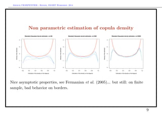
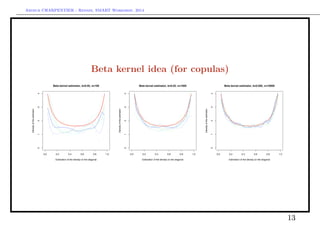
7. Arthur CHARPENTIER - Rennes, SMART Workshop, 2014
Non parametric estimation of copula density
see C., Fermanian & Scaillet (2005), bias of kernel estimators at endpoints
0.0 0.2 0.4 0.6 0.8 1.0
0.00.20.40.60.81.01.2
Kernel based estimation of the uniform density on [0,1]
Density
0.0 0.2 0.4 0.6 0.8 1.00.00.20.40.60.81.01.2
Kernel based estimation of the uniform density on [0,1]
Density
7

8. Arthur CHARPENTIER - Rennes, SMART Workshop, 2014
Non parametric estimation of copula density
e.g. E(c(0, 0, h)) =
1
4
· c(u, v) −
1
2
[c1(0, 0) + c2(0, 0)]
1
0
ωK(ω)dω · h + o(h)
0.2 0.4 0.6 0.8
0.2
0.4
0.6
0.8
0
1
2
3
4
5
Estimation of Frank copula
0.2 0.4 0.6 0.8
0.2
0.4
0.6
0.8
0
1
2
3
4
5
Estimation of Frank copula
0.0 0.2 0.4 0.6 0.8 1.0
0.00.20.40.60.81.0
with a symmetric kernel (here a Gaussian kernel).
8

9. Arthur CHARPENTIER - Rennes, SMART Workshop, 2014
Non parametric estimation of copula density
0.0 0.2 0.4 0.6 0.8 1.0
01234
Standard Gaussian kernel estimator, n=100
Estimation of the density on the diagonal
Densityoftheestimator
0.0 0.2 0.4 0.6 0.8 1.0
01234
Standard Gaussian kernel estimator, n=1000
Estimation of the density on the diagonal
Densityoftheestimator
0.0 0.2 0.4 0.6 0.8 1.0
01234
Standard Gaussian kernel estimator, n=10000
Estimation of the density on the diagonal
Densityoftheestimator
Nice asymptotic properties, see Fermanian et al. (2005)... but still: on finite
sample, bad behavior on borders.
9

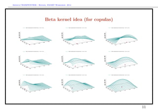
10. Arthur CHARPENTIER - Rennes, SMART Workshop, 2014
Beta kernel idea (for copulas)
see Chen (1999, 2000), Bouezmarni & Rolin (2003),
Kxi (u) ∝ exp −
(u − xi)2
h2
vs. Kxi (u) ∝ u
x1,i
b
1 [1 − u1]
x1,i
b · u
x2,i
b
2 [1 − u2]
x2,i
b
10
q
q
q
q
q
q
q
q
q
q
q
q
q
q
q
q
q
q
q
q
q
q
q
q
q
q q
q
q
q
q
q
q
q
q
q
q
q
q
q
q
q
q
q
q
q
q
q
q
q
q
q
q
q
q
q
q
q
q q
q
q
qq
q
q
q
q
q
qq
q
q
q
q
q
q
q
q
q
q
q q
q
q
q
q
q
q
q
q
q
q
q
q
q
q
q
q
q
q
q
q
q
q
q
q
q
q
q
q
q
q
q
q q
q
q
q
q q
q
q
q
q
q
q
q
q
q
q
q
q
q
q
qq
q
q
q
q
q
q
q
q
q
q
q
q
q
q
q
q
q
q
q
q
q
q
q
q q
q
q
q
q
q
q
q
q
q
q
q
q
q
q q
q
q
q
q
q
q
q
q
q
q
q
q
qq
q
q
q
q
q
q
q
q
q
q
q
q
q
q
q
q
q
q
qq
q
q
q
q
q
q
q
q
q
q
q
q
q
q
q
q
q
q
q
q
q
q
q
q
q
q
q
q
q
q
q
q
q
q
q
q
q
q
q
q
q
q
qq
qq
q
q
q
q q
q
q q
q
q
q
q
q
q
q
q
q
q
q
q
q
q
q
q
q
q
q
q
q
q
q
q
q
q
q
q
q
q
q
q
q
q
q
q
q
q
q
qq
q
q
q
q
q
q
q
q
q
q
q
q
q
q q
q
q
q
q
q
q
q
q
q
q
q
q
q
q
q
q
q
q
q
q
q
q
q
q
q q
q
q
q
q
q
q q
q
q
q
q
q
q
q
q
q
q
q
q
q
q
q
q
q
q
q
q
q
q
q q
q
q
q
q
q
q
q
q
q
q
q
q
q
q
q
q
q
q
q
q
q
q

11. Arthur CHARPENTIER - Rennes, SMART Workshop, 2014
Beta kernel idea (for copulas)
Beta (independent) bivariate kernel , x=0.0, y=0.0 Beta (independent) bivariate kernel , x=0.2, y=0.0 Beta (independent) bivariate kernel , x=0.5, y=0.0
Beta (independent) bivariate kernel , x=0.0, y=0.2 Beta (independent) bivariate kernel , x=0.2, y=0.2 Beta (independent) bivariate kernel , x=0.5, y=0.2
Beta (independent) bivariate kernel , x=0.0, y=0.5 Beta (independent) bivariate kernel , x=0.2, y=0.5 Beta (independent) bivariate kernel , x=0.5, y=0.5
11

12. Arthur CHARPENTIER - Rennes, SMART Workshop, 2014
Beta kernel idea (for copulas)
0.2 0.4 0.6 0.8
0.2
0.4
0.6
0.8
0
1
2
3
4
5
Estimation of Frank copula
0.2 0.4 0.6 0.8
0.2
0.4
0.6
0.8
0.0
0.5
1.0
1.5
2.0
2.5
3.0
Estimation of the copula density (Beta kernel, b=0.1)
0.2 0.4 0.6 0.8
0.2
0.4
0.6
0.8
0.0
0.5
1.0
1.5
2.0
2.5
3.0
Estimation of the copula density (Beta kernel, b=0.05)
12

13. Arthur CHARPENTIER - Rennes, SMART Workshop, 2014
Beta kernel idea (for copulas)
0.0 0.2 0.4 0.6 0.8 1.0
01234
Beta kernel estimator, b=0.05, n=100
Estimation of the density on the diagonal
Densityoftheestimator
0.0 0.2 0.4 0.6 0.8 1.0
01234
Beta kernel estimator, b=0.02, n=1000
Estimation of the density on the diagonal
Densityoftheestimator
0.0 0.2 0.4 0.6 0.8 1.0
01234
Beta kernel estimator, b=0.005, n=10000
Estimation of the density on the diagonal
Densityoftheestimator
13

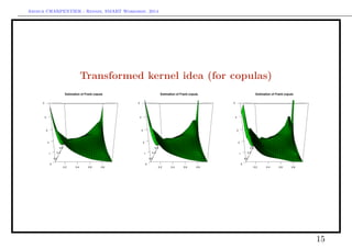
14. Arthur CHARPENTIER - Rennes, SMART Workshop, 2014
Transformed kernel idea (for copulas)
[0, 1] × [0, 1] → R × R → [0, 1] × [0, 1]
14

15. Arthur CHARPENTIER - Rennes, SMART Workshop, 2014
Transformed kernel idea (for copulas)
0.2 0.4 0.6 0.8
0.2
0.4
0.6
0.8
0
1
2
3
4
5
Estimation of Frank copula
0.2 0.4 0.6 0.8
0.2
0.4
0.6
0.8
0
1
2
3
4
5
Estimation of Frank copula
0.2 0.4 0.6 0.8
0.2
0.4
0.6
0.8
0
1
2
3
4
5
Estimation of Frank copula
15

16. Arthur CHARPENTIER - Rennes, SMART Workshop, 2014
Transformed kernel idea (for copulas)
0.0 0.2 0.4 0.6 0.8 1.0
01234
Transformed kernel estimator (Gaussian), n=100
Estimation of the density on the diagonal
Densityoftheestimator
0.0 0.2 0.4 0.6 0.8 1.0
01234
Transformed kernel estimator (Gaussian), n=1000
Estimation of the density on the diagonal
Densityoftheestimator
0.0 0.2 0.4 0.6 0.8 1.0
01234
Transformed kernel estimator (Gaussian), n=10000
Estimation of the density on the diagonal
Densityoftheestimator
see Geenens, C. & Paindaveine (2014) for more details on probit transformation
for copulas.
16

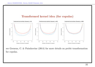
17. Arthur CHARPENTIER - Rennes, SMART Workshop, 2014
Combining the two approaches
See Devroye & Györfi (1985), and Devroye & Lugosi (2001)
... use the transformed kernel the other way, R → [0, 1] → R
17

18. Arthur CHARPENTIER - Rennes, SMART Workshop, 2014
Devroye & Györfi (1985) - Devroye & Lugosi (2001)
Interesting point, the optimal T should be F,
thus, T can be Fθ
18

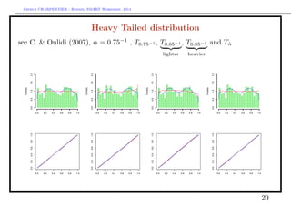
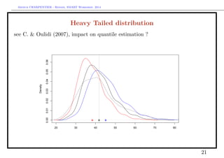
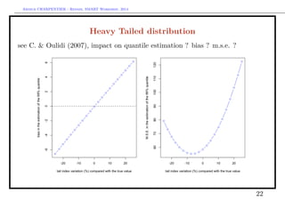
19. Arthur CHARPENTIER - Rennes, SMART Workshop, 2014
Heavy Tailed distribution
Let X denote a (heavy-tailed) random variable with tail index α ∈ (0, ∞), i.e.
P(X > x) = x−α
L1(x)
where L1 is some regularly varying function.
Let T denote a R → [0, 1] function, such that 1 − T is regularly varying at
infinity, with tail index β ∈ (0, ∞).
Define Q(x) = T−1
(1 − x−1
) the associated tail quantile function, then
Q(x) = x1/β
L2(1/x), where L2 is some regularly varying function (the de Bruyn
conjugate of the regular variation function associated with T). Assume here that
Q(x) = bx1/β
Let U = T(X). Then, as u → 1
P(U > u) ∼ (1 − u)α/β
.
19

20. Arthur CHARPENTIER - Rennes, SMART Workshop, 2014
Heavy Tailed distribution
see C. & Oulidi (2007), α = 0.75−1
, T0.75−1 , T0.65−1
lighter
, T0.85−1
heavier
and Tˆα
Density
0.0 0.2 0.4 0.6 0.8 1.0
0.00.51.01.52.0
0.0 0.2 0.4 0.6 0.8 1.0
0.00.20.40.60.81.0
Density
0.0 0.2 0.4 0.6 0.8 1.0
0.00.51.01.52.0
0.0 0.2 0.4 0.6 0.8 1.0
0.00.20.40.60.81.0
Density
0.0 0.2 0.4 0.6 0.8 1.0
0.00.51.01.52.0
0.0 0.2 0.4 0.6 0.8 1.0
0.00.20.40.60.81.0
Density
0.0 0.2 0.4 0.6 0.8 1.0
0.00.51.01.52.0
0.0 0.2 0.4 0.6 0.8 1.0
0.00.20.40.60.81.0
20

21. Arthur CHARPENTIER - Rennes, SMART Workshop, 2014
Heavy Tailed distribution
see C. & Oulidi (2007), impact on quantile estimation ?
20 30 40 50 60 70 80
0.000.010.020.030.040.050.06
Density
21

22. Arthur CHARPENTIER - Rennes, SMART Workshop, 2014
Heavy Tailed distribution
see C. & Oulidi (2007), impact on quantile estimation ? bias ? m.s.e. ?
22

23. Arthur CHARPENTIER - Rennes, SMART Workshop, 2014
Which transformation ?
GB2 : t(y; a, b, p, q) =
|a|yap−1
bapB(p, q)[1 + (y/b)a]p+q
, for y > 0,
GB2
q→∞

a=1
p=1
55
q=1
@@
GG
a→0
ÓÓ
a=1
p=1
%%
Beta2
q→∞
ww
SM
q→∞
xx
q=1
99
Dagum
p=1
Lognormal Gamma Weibull Champernowne
23

24. Arthur CHARPENTIER - Rennes, SMART Workshop, 2014
Estimating a density on R+
• Stay on R+ : xi’s
• Get on [0, 1] : ui = Tθ
(xi) (distribution as uniform as possible)
◦ Use Beta Kernels on ui’s
◦ Mixtures of Beta distributions on ui’s
◦ Bernstein Polynomials on ui’s
• Get on R : use standard kernels (e.g. Gaussian)
◦ On xi = log(xi)
◦ On xi = BoxCoxλ
(xi)
◦ On xi = Φ−1
[Tθ
(xi)]
24

25. Arthur CHARPENTIER - Rennes, SMART Workshop, 2014
Beta kernel
g(u) =
n
i=1
1
n
· b u;
Ui
h
,
1 − Ui
h
u ∈ [0, 1].
with some possible boundary correction, as suggested in Chen (1999),
u
h
→ ρ(u, h) = 2h2
+ 2.5 − (4h4
+ 6h2
+ 2.25 − u2
− u/h)1/2
Problem : choice of the bandwidth h ? Standard loss function
L(h) = [gn(u) − g(u)]2
du = [gn(u)]2
du − 2 gn(u) · g(u)du
CV (h)
+ [g(u)]2
du
where
CV (h) = gn(u)du
2
−
2
n
n
i=1
g(−i)(Ui)
25

26. Arthur CHARPENTIER - Rennes, SMART Workshop, 2014
Mixture of Beta distributions
g(u) =
k
j=1
πj · b u; αj, βj u ∈ [0, 1].
Problem : choice the number of components k (and estimation...). Use of
stochastic EM algorithm (or sort of) see Celeux Diebolt (1985).
Bernstein approximation
g(u) =
m
k=1
[mωk] · b (u; k, m − k) u ∈ [0, 1].
where ωk = G
k
m
− G
k − 1
m
.
26

27. Arthur CHARPENTIER - Rennes, SMART Workshop, 2014
On the log-transform
With a standard Gaussian kernel
fX(x) =
1
n
n
i=1
φ(x; xi, h)
A Gaussian kernel on a log transform,
fX(x) =
1
x
fX (log x) =
1
n
n
i=1
λ(x; log xi, h)
where λ(·; µ, σ) is the density of the log-normal distribution. Here, in 0,
bias[fX(x)] ∼
h2
2
[fX(x) + 3x · fX(x) + x2
· fX(x)]
and
Var[fX(x)] ∼
fX(x)
xnh
27

28. Arthur CHARPENTIER - Rennes, SMART Workshop, 2014
On the Box-Cox-transform
More generally, instead of transformed sample Yi = log[Xi], consider
Yi =
Xλ
i − 1
λ
when λ = 0.
Find the optimal transformation using standard regression techniques (least
squares)
Xi =
Xλ
i − 1
λ
when λ = 0
and Xi = log[Xi] if λ = 0. The density estimation is here
fX(x) = xλ −1
fX
xλ
− 1
λ
28

29. Arthur CHARPENTIER - Rennes, SMART Workshop, 2014
Illustration with Log-normal samples
Standard kernel (− Silvermans’s rule h )
Density
0 2 4 6 8 10 12
0.00.10.20.30.40.50.6
Density
0 2 4 6 8 10 12
0.00.10.20.30.40.50.6
Density
0 2 4 6 8 10 12
0.00.10.20.30.40.50.6
29

30. Arthur CHARPENTIER - Rennes, SMART Workshop, 2014
Illustration with Log-normal samples
Log transform, xi = log xi + Gaussian kernel
Density
−2 −1 0 1 2
0.00.10.20.30.40.50.6
Density
−2 −1 0 1 20.00.10.20.30.40.50.6
Density
−2 −1 0 1 2
0.00.10.20.30.40.50.6
Density
0 2 4 6 8 10 12
0.00.10.20.30.40.50.6
Density
0 2 4 6 8 10 12
0.00.10.20.30.40.50.6
Density
0 2 4 6 8 10 12
0.00.10.20.30.40.50.6
30

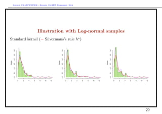
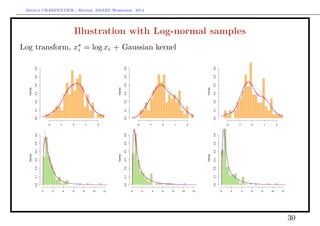
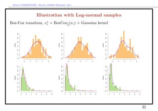
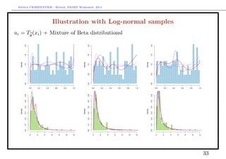
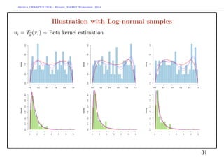
31. Arthur CHARPENTIER - Rennes, SMART Workshop, 2014
Illustration with Log-normal samples
Probit-type transform, xi = Φ−1
[Tθ
(xi)] + Gaussian kernel
Density
−2 −1 0 1 2
0.00.10.20.30.40.50.6
Density
−2 −1 0 1 20.00.10.20.30.40.50.6
Density
−2 −1 0 1 2
0.00.10.20.30.40.50.6
Density
0 2 4 6 8 10 12
0.00.10.20.30.40.50.6
Density
0 2 4 6 8 10 12
0.00.10.20.30.40.50.6
Density
0 2 4 6 8 10 12
0.00.10.20.30.40.50.6
31

32. Arthur CHARPENTIER - Rennes, SMART Workshop, 2014
Illustration with Log-normal samples
Box-Cox transform, xi = BoxCoxλ
(xi) + Gaussian kernel
Density
−2 −1 0 1 2
0.00.10.20.30.40.50.6
Density
−2 −1 0 1 20.00.10.20.30.40.50.6
Density
−2 −1 0 1 2
0.00.10.20.30.40.50.6
Density
0 2 4 6 8 10 12
0.00.10.20.30.40.50.6
Density
0 2 4 6 8 10 12
0.00.10.20.30.40.50.6
Density
0 2 4 6 8 10 12
0.00.10.20.30.40.50.6
32

33. Arthur CHARPENTIER - Rennes, SMART Workshop, 2014
Illustration with Log-normal samples
ui = Tθ
(xi) + Mixture of Beta distributionsl
Density
0.0 0.2 0.4 0.6 0.8 1.0
0.00.51.01.52.0
Density
0.0 0.2 0.4 0.6 0.8 1.00.00.51.01.52.0
Density
0.0 0.2 0.4 0.6 0.8 1.0
0.00.51.01.52.0
Density
0 2 4 6 8 10 12
0.00.10.20.30.40.50.6
Density
0 2 4 6 8 10 12
0.00.10.20.30.40.50.6
Density
0 2 4 6 8 10 12
0.00.10.20.30.40.50.6
33

34. Arthur CHARPENTIER - Rennes, SMART Workshop, 2014
Illustration with Log-normal samples
ui = Tθ
(xi) + Beta kernel estimation
Density
0.0 0.2 0.4 0.6 0.8 1.0
0.00.51.01.52.0
Density
0.0 0.2 0.4 0.6 0.8 1.00.00.51.01.52.0
Density
0.0 0.2 0.4 0.6 0.8 1.0
0.00.51.01.52.0
Density
0 2 4 6 8 10 12
0.00.10.20.30.40.50.6
Density
0 2 4 6 8 10 12
0.00.10.20.30.40.50.6
Density
0 2 4 6 8 10 12
0.00.10.20.30.40.50.6
34

35. Arthur CHARPENTIER - Rennes, SMART Workshop, 2014
Quantities of interest
Standard statistical quantities
• miae,
∞
0
fn(x) − f(x) dx
• mise,
∞
0
fn(x) − f(x)
2
dx
• miaew,
∞
0
fn(x) − f(x) |x| dx
• misew,
∞
0
fn(x) − f(x)
2
x2
dx
35

36. Arthur CHARPENTIER - Rennes, SMART Workshop, 2014
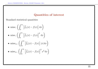
Quantities of interest
Inequality indices and risk measures, based on F(x) =
x
0
f(t)dt,
• Gini,
1
µ
∞
0
F(t)[1 − F(t)]dt
• Theil,
∞
0
t
µ
log
t
µ
f(t)dt
• Entropy −
∞
0
f(t) log[f(t)]dt
• VaR-quantile, x such that F(x) = P(X ≤ x) = α, i.e. F−1
(α)
• TVaR-expected shorfall, E[X|X F−1
(α)]
where µ =
∞
0
[1 − F(x)]dx.
36

37. Arthur CHARPENTIER - Rennes, SMART Workshop, 2014
Computations Aspects
Here, for each method, we return two functions,
• function fn(·)
• a random generator for distribution fn(·)
◦ H-transform and Gaussian kernel
draw i ∈ {1, · · · , n} and X = H−1
(Z) where Z ∼ N(H(xi), b2
)
◦ H-transform and Beta kernel
draw i ∈ {1, · · · , n} and X = H−1
(U) where U ∼ B(H(xi)/h, [1 − H(xi)]/h)
◦ H-transform and Beta mixture
draw k ∈ {1, · · · , K} and X = H−1
(U) where U ∼ B(αk, βk)
37

38. Arthur CHARPENTIER - Rennes, SMART Workshop, 2014
◦ ‘standard’ Gaussian kernel (benchmark)
draw i ∈ {1, · · · , n}, and X ∼ N(xi, b2
) (almost)
up to some normalization, · →
fn(·)
∞
0
fn(x)dx
38
Density
−2 0 2 4 6 8
0.00.10.20.30.4
q qq qqq q qqq

39. Arthur CHARPENTIER - Rennes, SMART Workshop, 2014
MISE
∞
0
f(s)
n (x) − f(x)
2
dx
q
Singh−Maddala
MISE
qqq qq
qqqqqq q
q qqq qq qqq qq q
qqqq qq q
q qqq qq qqq qq q
qqqq qq q q
qqq qq
qq qq q qq qqq q
standard kernel
log kernel
log mix
boxcox kernel
boxcox mix
probit kernel
beta kernel
beta mix
0.000
0.005
0.010
0.015
q
Mixed Singh−Maddala
MISE
qq
q qqq qqq qqq q
q qq qqq qq qqq q
q qq qq qqq qq qqqq q
qqq qq
qqq
standard kernel
log kernel
log mix
boxcox kernel
boxcox mix
probit kernel
beta kernel
beta mix
0.00
0.05
0.10
0.15
39

40. Arthur CHARPENTIER - Rennes, SMART Workshop, 2014
MIAE
∞
0
|f(s)
n (x) − f(x)| dx
q
Singh−Maddala
MIAE
q qqq q
qq qq qq
q qq
qqqq qq
q qq qq
qqqq q
qq qqq q
q qqq
standard kernel
log kernel
log mix
boxcox kernel
boxcox mix
probit kernel
beta kernel
beta mix
0.00
0.05
0.10
0.15
0.20
q
Mixed Singh−Maddala
MIAE
q
qq q
q qqqqq q
q q
standard kernel
log kernel
log mix
boxcox kernel
boxcox mix
probit kernel
beta kernel
beta mix
0.05
0.10
0.15
0.20
0.25
0.30
40

41. Arthur CHARPENTIER - Rennes, SMART Workshop, 2014
Gini Index
1
µ
(s)
n
∞
0
F(s)
n (t)[1 − F(s)
n (t)]dt
Singh−Maddala
Gini Index
q q
qq
q q
qq
q
qqq
q q
standard kernel
log kernel
log mix
boxcox kernel
boxcox mix
probit kernel
beta kernel
beta mix
0.45
0.50
0.55
0.60
Mixed Singh−Maddala
Gini Index
q
qq
q
q
q qq
qq
standard kernel
log kernel
log mix
boxcox kernel
boxcox mix
probit kernel
beta kernel
beta mix
0.55
0.60
0.65
0.70
41

42. Arthur CHARPENTIER - Rennes, SMART Workshop, 2014
Value-at-Risk, 95%
Q(s)
n (α) = inf{x, α ≤ F(s)
n (x)}
q
Singh−Maddala
Quantile 95%
qq qqqq q
q q qq q
qq
q qqqqq q
q qqqqqq qq
qq qqqqqq
qqq q
qq
standard kernel
log kernel
log mix
boxcox kernel
boxcox mix
probit kernel
beta kernel
beta mix
10
20
30
40
50
Mixed Singh−Maddala
Quantile 95%
qq
q q
q
q
q q
q
standard kernel
log kernel
log mix
boxcox kernel
boxcox mix
probit kernel
beta kernel
beta mix
2.0
2.5
3.0
3.5
4.0
4.5
42

43. Arthur CHARPENTIER - Rennes, SMART Workshop, 2014
Value-at-Risk, 99%
Q(s)
n (α) = inf{x, α ≤ F(s)
n (x)}
Singh−Maddala
Quantile 99%
q qqq
qq q qqq
qq
qqq qq qqqq
qq qqqq
qq qqqq
qq q
qq
standard kernel
log kernel
log mix
boxcox kernel
boxcox mix
probit kernel
beta kernel
beta mix
6
8
10
12
14
16
18
q
Mixed Singh−Maddala
Quantile 99%
q q
q qqqqqq qqqq
qqq qqq
q qqqqq
q q qq
qq q
standard kernel
log kernel
log mix
boxcox kernel
boxcox mix
probit kernel
beta kernel
beta mix
2
4
6
8
10
43

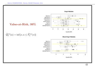
44. Arthur CHARPENTIER - Rennes, SMART Workshop, 2014
Tail Value-at-Risk, 95%
E[X|X Q(s)
n (α)]
Singh−Maddala
Expected Shortfall 95%
q
q
qq
q
qq
q
standard kernel
log kernel
log mix
boxcox kernel
boxcox mix
probit kernel
beta kernel
beta mix
4.0
4.5
5.0
5.5
6.0
6.5
q
Mixed Singh−Maddala
Expected Shortfall 95%
q qqq
q qqq
q qqq
q qqq
q
standard kernel
log kernel
log mix
boxcox kernel
boxcox mix
probit kernel
beta kernel
beta mix
4
6
8
10
12
44

45. Arthur CHARPENTIER - Rennes, SMART Workshop, 2014
Possible conclusion ?
• estimating densities on transformated data is definitively a good idea
• but we need to find a good transformation
parametric + beta
parametric + probit
log-transform
Box-Cox
0.719
0.719
0.719
0.719
0.719
0.719
0.719
0.719
1.428
2.137
47.75
48.00
48.25
48.50
48.75
−4.8 −4.4 −4.0 −3.6
longitude
latitude
0.011
0.719
1.428
2.137
2.845
0.719
0.719
0.7190.719
0.719
0.719
0.719
0.719
0.719
1.428
1.428
1.428
1.428
1.428
1.4281.428
1.428
1.428
1.428
1.428
1.428
1.428
1.428
1.428
1.428
2.137
2.137
47.75
48.00
48.25
48.50
48.75
−4.8 −4.4 −4.0 −3.6
longitude
latitude 0.011
0.719
1.428
2.137
2.845
(joint work with E. Gallic)
45