Side 2019 #5

Arthur Charpentier, SIDE Summer School, July 2019
# 5 Classification & Boosting
Arthur Charpentier (Université du Québec à Montréal)
Machine Learning & Econometrics
SIDE Summer School - July 2019
@freakonometrics freakonometrics freakonometrics.hypotheses.org 1

Starting Point: Classification Tree
1 library(rpart)
2 cart = rpart(PRONO˜.,data=
myocarde)
3 library(rpart.plot)
4 prp(cart ,type=2, extra =1)
A (binary) split is based on one specific variable âĂŞ say xj âĂŞ and a cutoff,
say s. Then, there are two options:
• either xi,j ≤ s, then observation i goes on the left, in IL
• or xi,j > s, then observation i goes on the right, in IR
Thus, I = IL ∪ IR.

Classification : Classification Trees
Gini for node I is defined as
G(I) = −
y∈{0,1}
py(1 − py)
where py is the proportion of individuals in the leaf of type y,
G(I) = −
y∈{0,1}
ny,I
nI
1 −
ny,I
nI
1 gini = function(y,classe){
2 T. = table(y,classe)
3 nx = apply(T,2,sum)
4 n. = sum(T)
5 pxy = T/matrix(rep(nx ,each =2) ,nrow =2)
6 omega = matrix(rep(nx ,each =2) ,nrow =2)/n
7 g. = -sum(omega*pxy*(1-pxy))
8 return(g)}

1 -2*mean(myocarde$PRONO)*(1-mean(myocarde$PRONO))
2 [1] -0.4832375
3 gini(y=myocarde$PRONO ,classe=myocarde$PRONO <Inf)
4 [1] -0.4832375
5 gini(y=myocarde$PRONO ,classe=myocarde [ ,1] <=100)
6 [1] -0.4640415

if we split, deﬁne index
G(IL, IR) = −
x∈{L,R}
nx
nIx
nI
y∈{0,1}
ny,Ix
nIx
1 −
ny,Ix
nIx
the entropic measure is
E(I) = −
y∈{0,1}
ny,I
nI
log
ny,I
nI
1 entropy = function(y,classe){
2 T = table(y,classe)
3 nx = apply(T,2,sum)
4 pxy = T/matrix(rep(nx ,each =2) ,nrow =2)
5 omega = matrix(rep(nx ,each =2) ,nrow =2)/sum(T)
6 g = sum(omega*pxy*log(pxy))
7 return(g)}

1 mat_gini = mat_v=matrix(NA ,7 ,101)
2 for(v in 1:7){
3 variable=myocarde[,v]
4 v_seuil=seq(quantile(myocarde[,v],
5 6/length(myocarde[,v])),
6 quantile(myocarde[,v],1-6/length(
7 myocarde[,v])),length =101)
8 mat_v[v,]=v_seuil
9 for(i in 1:101){
10 CLASSE=variable <=v_seuil[i]
11 mat_gini[v,i]=
12 gini(y=myocarde$PRONO ,classe=CLASSE)}}
13 -(gini(y=myocarde$PRONO ,classe =( myocarde
[ ,3] <19))-
14 gini(y=myocarde$PRONO ,classe =( myocarde [,3]<
Inf)))/
15 gini(y=myocarde$PRONO ,classe =( myocarde [,3]<
Inf))
16 [1] 0.5862131

1 idx = which(myocarde$INSYS <19)
2 mat_gini = mat_v = matrix(NA ,7 ,101)
3 for(v in 1:7){
4 variable = myocarde[idx ,v]
5 v_seuil = seq(quantile(myocarde[idx ,v],
6 7/length(myocarde[idx ,v])),
7 quantile(myocarde[idx ,v],1-7/length(
8 myocarde[idx ,v])), length =101)
9 mat_v[v,] = v_seuil
10 for(i in 1:101){
11 CLASSE = variable <=v_seuil[i]
12 mat_gini[v,i]=
13 gini(y=myocarde$PRONO[idx],classe=
CLASSE)}}
14 par(mfrow=c(3 ,2))
15 for(v in 2:7){
16 plot(mat_v[v,],mat_gini[v ,])
17 }

1 idx = which(myocarde$INSYS >=19)
2 mat_gini = mat_v = matrix(NA ,7 ,101)
3 for(v in 1:7){
4 variable=myocarde[idx ,v]
5 v_seuil=seq(quantile(myocarde[idx ,v],
6 6/length(myocarde[idx ,v])),
7 quantile(myocarde[idx ,v],1-6/length(
8 myocarde[idx ,v])), length =101)
9 mat_v[v,]=v_seuil
10 for(i in 1:101){
11 CLASSE=variable <=v_seuil[i]
12 mat_gini[v,i]=
13 gini(y=myocarde$PRONO[idx],
14 classe=CLASSE)}}
15 par(mfrow=c(3 ,2))
16 for(v in 2:7){
17 plot(mat_v[v,],mat_gini[v ,])
18 }

Boosting & Adaboost
Classiﬁcation problem, yi ∈ {•, •}, consider a model at stage
k − 1,
if mk−1(xi) = yi, increase the weight given to observation i
Boosting : weak learner
A weak model is a model slightly better than a pure
random one (head/tails)
q
q
q
q
q
q
q
q
q
q
0.0 0.2 0.4 0.6 0.8 1.0
0.00.20.40.60.81.0
0.5
q
q
q
q
q
q
q
q
q
q
q
q
q
q
q
q
q
q
0.0 0.2 0.4 0.6 0.8 1.0
0.00.20.40.60.81.0
0.5q
q
q
q
q
q
q
q
q

Boosting & Adaboost
Classiﬁcation problem, yi ∈ {•, •}, consider a model at stage
k − 1,
if mk−1(xi) = yi, increase the weight given to observation i
Boosting : weak learner
A weak model is a model slightly better than a pure
random one (head/tails)
q
q
q
q
q
q
q
q
q
q
0.0 0.2 0.4 0.6 0.8 1.0
0.00.20.40.60.81.0
0.5
q
q
q
q
q
q
q
q
q
q
q
q
q
q
q
q
q
q
0.0 0.2 0.4 0.6 0.8 1.0
0.00.20.40.60.81.0
0.5
q
q
q
q
q
q
q
q
q
q

Boosting & Adaboost
Adaboost Algorithm
1. Set weights ωi = 1/n, i = 1, · · · , n
2 . For k = 1, · · ·
(i) ﬁt model on (yi, xi) with weights ωi, get hk(x)
(ii) compute the error rate εk =
n
i=1
˜ωi1yi=hk(xi)
(iii) compute αk = log
1 − εk
εk
(iv) reevaluate the weights ωi = ωi · eαk1yi=hk(xi)
3. The ﬁnal model is hκ(x) =
κ
k≥1
αkhk(x)
The error rate should not be too small (εk ≤ 50%) to insure αk > 0

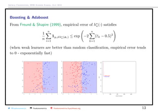
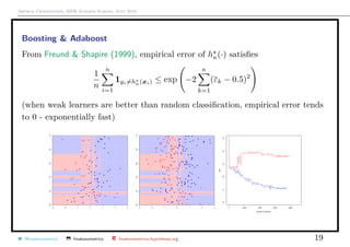
Boosting & Adaboost
The general problem in machine learning is to ﬁnd m (·) = argmin
m∈M
E (Y, g(X)
Use loss (y, g(x)) = 1y=g(x.
Empirical version is mn(·) = argmin
m∈M
1
n
n
i=1
(yi, g(xi) = argmin
m∈M
1
n
n
i=1
1yi=g(xi)
Complicated problem : use a convex version of the loss function
(y, g(x) = exp[−y · g(x)]
From Hastie et al. (2009), with the adaboost algorithm,
hκ(·) = hκ−1(·) + ακhκ(x) = hκ−1(·) + 2β H (·)
where (β , H (·)) = argmin
(β,H)∈(R,M)
n
i=1
exp − yi · (hκ−1(xi) + βH(xi)

Boosting & Adaboost
From Freund & Shapire (1999), empirical error of hκ(·) satisﬁes
1
n
n
i=1
1yi=hκ(xi) ≤ exp −2
κ
k=1
(εk − 0.5)2
(when weak learners are better than random classiﬁcation, empirical error tends
to 0 - exponentially fast)
−3 −2 −1 0 1 2 3
0.00.20.40.60.81.0
q
q
q
q
q
q
q
q
q
q
q
q
q
q
q
q
q
qq
q
q
q
q
q
q
q
q
q
q
q
q
q
q
q
q
qq
q
q
q
q
q
q
q
q
q
q
q
q
q
q
q
q
q
q
q
q
q
q
q
q
q
q
q
q
q
q
q
q
q
q
q
q
q
q
q
q
q
q
q
q
q
q
q
q
q
q
q
q
qq
q
q
q
q
q
q
q
q
q
−3 −2 −1 0 1 2 3
0.00.20.40.60.81.0
q
q
q
q
q
q
q
q
q
q
q
q
q
q
q
q
q
q
q
q
q
q
q
q
q
q
q
q
q
q
q
q
q
q
q
q
q
q
q
q
q
q
q
q
q
q
q
q
q
q
q
q
q
q
q
q
q
q
q
q
q
q
q
q
q
q
q
q
q
q
q
q
q
q
q
q
q
q
q
q
q
q
q
q
q
q
q
q
q
q
q
q
q
q
q
q
q
q
q
q
q
q
q
q
q
q
q
q
q
q
q
q
q
q
q
q
q
q
q
q
q
q
q
q
q
q
q
q
q
q
q
q
q
q
q
q
q
q
q
q
q
q
q
q
q
q
q
q
q
q
q
q
q
q
q
q
q
q
q
q
q
qq
q
q
q
q
q
q
q
q
q
q
q
q
q
q
q
q
q
q
q
q
q
q
q
q
q
q
q
q
q
q
q
qq
q
q
q
q
0 2000 4000 6000 8000
0.00.10.20.30.40.5
Number of iterations
Error
training sample
validation sample

Boosting & Adaboost
1
n
n
i=1
κ
k=1
(εk − 0.5)2
−3 −2 −1 0 1 2 3
0.00.20.40.60.81.0
q
q
q
q
q
q
q
q
q
q
q
q
q
q
q
q
q
qq
q
q
q
q
q
q
q
q
q
q
q
q
q
q
q
q
qq
q
q
q
q
q
q
q
q
q
q
q
q
q
q
q
q
q
q
q
q
q
q
q
q
q
q
q
q
q
q
q
q
q
q
q
q
q
q
q
q
q
q
q
q
q
q
q
q
q
q
q
q
qq
q
q
q
q
q
q
q
q
q
−3 −2 −1 0 1 2 3
0.00.20.40.60.81.0
q
q
q
q
q
q
q
q
q
q
q
q
q
q
q
q
q
q
q
q
q
q
q
q
q
q
q
q
q
q
q
q
q
q
q
q
q
q
q
q
q
q
q
q
q
q
q
q
q
q
q
q
q
q
q
q
q
q
q
q
q
q
q
q
q
q
q
q
q
q
q
q
q
q
q
q
q
q
q
q
q
q
q
q
q
q
q
q
q
q
q
q
q
q
q
q
q
q
q
q
q
q
q
q
q
q
q
q
q
q
q
q
q
q
q
q
q
q
q
q
q
q
q
q
q
q
q
q
q
q
q
q
q
q
q
q
q
q
q
q
q
q
q
q
q
q
q
q
q
q
q
q
q
q
q
q
q
q
q
q
q
qq
q
q
q
q
q
q
q
q
q
q
q
q
q
q
q
q
q
q
q
q
q
q
q
q
q
q
q
q
q
q
q
qq
q
q
q
q
0 2000 4000 6000 8000
0.00.10.20.30.40.5
Error
training sample
validation sample

Gradient Boosting
Newton-Raphson to minimize a strictly convex function g : R → R
At minimum, g (x ) = 0, so consider ﬁrst order approximation
g (x + h) ≈ g (x) + h · g (x)
Consider sequence xk = xk−1 − αg (xk−1) where α = [g (xk−1)]−1
One can consider a functional version of that technique, ∀i = 1, · · · , n,
gk(xi) = gk−1(xi) − α
∂ (yi, g(xi))
∂g(xi) g(xi)=gk−1(xi)
This provides a sequence of function gk at points xi.
To get values at any point x use regression i’s on xi’s,
εi = −
∂ (yi, g))
∂g g=gk−1(xi)
If α = 1 and (y, g) = exp[−yg], we have (almost) adaboost

Gradient Boosting
Gradient Boosting Algorithm
1. Start with a constant model, h0(x) = argmin
c∈R
1
n
n
i=1
(yi, c) and a regu-
larization parameter α ∈ (0, 1)
2 . For k = 1, · · ·
(i) compute εi = −
∂ (yi, g))
∂g g=gk−1(xi)
(ii) ﬁt the (weak) model on sample (εi, xi) and let Hk denote the mode
(iii) update the model hk(·) = hk−1(·) + αHk(·)
3. The ﬁnal model is hκ(x)
The choice of α is (somehow) not important : use α ∼ 10%

Gradient Boosting
The logiboost model is obtained when y ∈ {0, 1} and loss function is
(y, m) = log[1 + exp(−2(2y − 1)m)]
Boosting (learning from the mistakes)
Sequential Learning
mk(·) = mk−1(·) + α · argmin
h∈H



n
i=1
yi − mk−1(xi)
εi
, h(xi)



Hence, learning is sequential, as opposed to bagging...

Bagging
Gradient Boosting Algorithm
1. For k = 1, · · ·
(i) draw a bootstrap sample from (yi, xi)’s
(ii) estimate a model mk on that sample
2. The ﬁnal model is m (·) =
1
κ
κ
i=1
mk(·)
To illustrate, suppose that m is some parametric model mθ.
mk = mθk
, obtained some sample Sk = {(yi, xi), i ∈ Ik}.
Let σ2
(x) = Var[mθ
(x)] and ρ(x) = Corr[mθ1
(x), mθ2
(x)] obtained on two
ramdom boostrap samples
Var[m (x)] = ρ(x)σ2
(x) +
1 − ρ(x)
κ
σ2
(x)

Gradient Boosting & Computational Issues
We have used (y, g(x) = exp[−y · m(x)] instead of 1y=m(x.
Misclassification error is (upper) bounded by the exponential loss
1
n
n
i=1
1yi·m(xi
≤
1
n
n
i=1
exp[−yi · m(xi]
Here m(x) is a linear combination of weak classifier, m(x) =
κ
j=1
αjhj(x).
Let M = [Mi,j] where Mi,j = yi · hj(xi) ∈ {−1, +1}, i.e. Mi,j = 1 whenever
(weak) classifier j correctly classifies individual i.
yi · m(xi) =
κ
j=1
αjyihj(xi) = Mα i
thus, R(α) =
1
n
n
i=1
exp[−yi · m(xi)] =
1
n
n
i=1
exp − (Mα)i

One can use coordinate descent, in direction j in which the directional derivative
is the steepest,
j ∈ argmin −
∂R(α + aej)
∂a a=0
where the objective can be written
−
∂
∂a
1
n
n
i=1
exp − (Mα)i − a(Mej)i
a=0
=
1
n
n
i=1
Mij exp − (Mα)i
Then
j ∈ argmin (d M)j where di =
exp[−(Mα)i]
i exp[−(Mα)i]

Then do a line-search to see how far we should go. The derivative is null if
−
∂R(α + aej)
∂a
= 0 i.e. a =
1
2
log
d+
=
1
2
log
1 − d−
d−
where d− =
i:Mi,j =−1
di and d+ =
i:Mi,j =+1
di.
Coordinate Descent Algorithm
1. di = 1/n for i = 1, · · · , n and α = 0
2 . For k = 1, · · ·
(i) ﬁnd optimal direction j ∈ argmin (d M)j
(ii) compute − =
i:Mi,j =−1
di and ak =
1
2
log
1 − d−
d−
(iii) set α = α + akej and di =
exp[−(Mα)i]
i exp[−(Mα)i]

very close to Adaboost : αj is the sum of ak where direction j was considered,
αj =
κ
k=1
ak1j (k)=j
Thus
m (x) =
κ
k=1
αjhj(x) =
κ
k=1
akhj (k)(x)
With Adaboost, we go in the same direction, with the same intensity : Adaboost
is equivalent to minimizing the exponential loss by coordinate descent.
Thus, we seek m (·) = argmin E(Y,X)∼F
exp (−Y · m(X))
which is minimized at m (x) =
1
2
log
P[Y = +1|X = x]
P[Y = −1|X = x]
(very close to the logistic regression)

Several packages can be used with R, such as adabag::boosting
1 library(adabag)
2 library(caret)
3 indexes= createDataPartition (myocarde$PRONO , p=.70 , list = FALSE)
4 train = myocarde[indexes , ]
5 test = myocarde[-indexes , ]
6 model = boosting(PRONO˜., data=train , boos=TRUE , mfinal =50)
7 pred = predict(model , test)
8 print(pred$confusion)
9 Observed Class
10 Predicted Class DECES SURVIE
11 DECES 5 0
12 SURVIE 3 12
or use cross-validation
1 cvmodel = boosting.cv(PRONO˜., data=myocarde , boos=TRUE , mfinal =10, v
=5)

or xgboost::xgboost
1 library(xgboost)
2 library(caret)
3 train_x = data.matrix(train [,-8])
4 train_y = train [,8]
5 test_x = data.matrix(test [,-8])
6 test_y = test [,8]
7 xgb_train = xgb.DMatrix(data=train_x, label=train_y)
8 xgb_test = xgb.DMatrix(data=test_x, label=test_y)
9 xgbc = xgboost(data=xgb_train , max.depth =3, nrounds =50)
10 pred = predict(xgbc , xgb_test)
11 pred_y = as.factor (( levels(test_y))[round(pred)])
12 (cm = e1071 :: confusionMatrix (test_y, pred_y))
13 Reference
14 Prediction DECES SURVIE
15 DECES 6 2
16 SURVIE 0 12

or gbm::gbm
1 library(gbm)
2 library(caret)
3 mod_gbm = gbm(PRONO =="SURVIE" ˜.,
4 data = train ,
5 distribution = "bernoulli",
6 cv.folds = 7,
7 shrinkage = .01,
8 n. minobsinnode = 10,
9 n.trees = 200)
10 pred = predict.gbm(object = mod_gbm ,
11 newdata = test ,
12 n.trees = 200,
13 type = "response")

Side 2019 #5

More Related Content

What's hot

Similar to Side 2019 #5

More from Arthur Charpentier

Recently uploaded

Side 2019 #5