Downloaded 52 times


![Arthur CHARPENTIER, Advanced Econometrics Graduate Course, Winter 2017, Université de Rennes 1
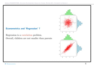
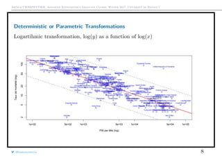
Econometrics and ‘Regression’ ?
1 > library(HistData)
2 > attach(Galton)
3 > Galton$count <- 1
4 > df <- aggregate(Galton , by=list(parent ,
child), FUN=sum)[,c(1,2,5)]
5 > plot(df[,1:2], cex=sqrt(df[,3]/3))
6 > abline(a=0,b=1,lty =2)
7 > abline(lm(child~parent ,data=Galton))
8 > coefficients (lm(child~parent ,data=Galton)
)[2]
9 parent
10 0.6462906
q q q q q
q q q
q q q q q q q q
q q q q q q q
q q
q q
q q q q q
q q q q q q q q q
q q q q q q q q q
q
q q q q q q q q
q q q q q q q q q
q q q q q q q q
q q q q q q q
q q q q q q q q
q q q q q q
q q q q
64 66 68 70 72
62646668707274
height of the mid−parent
heightofthechild
q q q q q
q q q
q q q q q q q q
q q q q q q q
q q
q q
q q q q q
q q q q q q q q q
q q q q q q q q q
q
q q q q q q q q
q q q q q q q q q
q q q q q q q q
q q q q q q q
q q q q q q q q
q q q q q q
q q q q
It is more an autoregression issue here :
if Yt = φYt−1 + εt cor[Yt, Yt+h] = φh
→ 0 as h → ∞.
@freakonometrics 3](https://image.slidesharecdn.com/slides-econometrics-2017-graduate-1-170209234511/85/Econometrics-PhD-Course-1-Nonlinearities-3-320.jpg)

![Arthur CHARPENTIER, Advanced Econometrics Graduate Course, Winter 2017, Université de Rennes 1
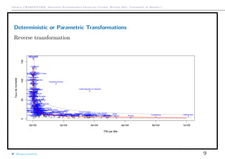
Box-Cox transformation
See Box & Cox (1964) An Analysis of Transformations ,
h(y, λ) =
yλ
− 1
λ
if λ = 0
log(y) if λ = 0
or
h(y, λ, µ) =
[y + µ]λ
− 1
λ
if λ = 0
log([y + µ]) if λ = 0
@freakonometrics 10
0 1 2 3 4
−4−3−2−1012
−1 −0.5 0 0.5 1 1.5 2](https://image.slidesharecdn.com/slides-econometrics-2017-graduate-1-170209234511/85/Econometrics-PhD-Course-1-Nonlinearities-10-320.jpg)
![Arthur CHARPENTIER, Advanced Econometrics Graduate Course, Winter 2017, Université de Rennes 1
Profile Likelihood
In a statistical context, suppose that unknown parameter can be partitioned
θ = (λ, β) where λ is the parameter of interest, and β is a nuisance parameter.
Consider {y1, · · · , yn}, a sample from distribution Fθ, so that the log-likelihood is
log L(θ) =
n
i=1
log fθ(yi)
θ
MLE
is defined as θ
MLE
= argmax {log L(θ)}
Rewrite the log-likelihood as log L(θ) = log Lλ(β). Define
β
pMLE
λ = argmax
β
{log Lλ(β)}
and then λpMLE
= argmax
λ
log Lλ(β
pMLE
λ ) . Observe that
√
n(λpMLE
− λ)
L
−→ N(0, [Iλ,λ − Iλ,βI−1
β,βIβ,λ]−1
)
@freakonometrics 11](https://image.slidesharecdn.com/slides-econometrics-2017-graduate-1-170209234511/85/Econometrics-PhD-Course-1-Nonlinearities-11-320.jpg)
![Arthur CHARPENTIER, Advanced Econometrics Graduate Course, Winter 2017, Université de Rennes 1
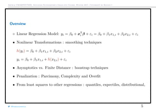
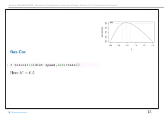
Uncertainty: Parameters vs. Prediction
Uncertainty on regression parameters (β0, β1)
From the output of the regression we can derive
confidence intervals for β0 and β1, usually
βk ∈ βk ± u1−α/2se[βk]
q
q
q
q
q
q
q
q
q
q
q
q
q
q
q
q
qq
q
q
q
q
q
q
q
q
q
q
q
q
q
q
q
q
q
q
q
q
q
q
q
q
q
q
q
q
qq
q
q
5 10 15 20 25
020406080100120
Vitesse du véhicule
Distancedefreinage
q
q
q
q
q
q
q
q
q
q
q
q
q
q
q
q
qq
q
q
q
q
q
q
q
q
q
q
q
q
q
q
q
q
q
q
q
q
q
q
q
q
q
q
q
q
qq
q
q
5 10 15 20 25
020406080100120
Vitesse du véhicule
Distancedefreinage
@freakonometrics 14](https://image.slidesharecdn.com/slides-econometrics-2017-graduate-1-170209234511/85/Econometrics-PhD-Course-1-Nonlinearities-14-320.jpg)
![Arthur CHARPENTIER, Advanced Econometrics Graduate Course, Winter 2017, Université de Rennes 1
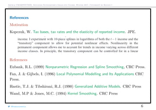
Uncertainty: Parameters vs. Prediction
Uncertainty on a prediction, y = m(x). Usually
m(x) ∈ m(x) ± u1−α/2se[m(x)]
hence, for a linear model
xT
β ± u1−α/2σ xT[XT
X]−1x
i.e. (with one covariate)
se2
[m(x)]2
= Var[β0 + β1x]
se2
[β0] + cov[β0, β1]x + se2
[β1]x2
q
q
q
q
q
q
q
q
q
q
q
q
q
q
q
q
qq
q
q
q
q
q
q
q
q
q
q
q
q
q
q
q
q
q
q
q
q
q
q
q
q
q
q
q
q
qq
q
q
5 10 15 20 25
020406080100120
Vitesse du véhicule
Distancedefreinage
1 > predict(lm(dist~speed ,data=cars),newdata=data.frame(speed=x),
interval="confidence")
@freakonometrics 15](https://image.slidesharecdn.com/slides-econometrics-2017-graduate-1-170209234511/85/Econometrics-PhD-Course-1-Nonlinearities-15-320.jpg)
![Arthur CHARPENTIER, Advanced Econometrics Graduate Course, Winter 2017, Université de Rennes 1
Least Squares and Expected Value (Orthogonal Projection Theorem)
Let y ∈ Rd
, y = argmin
m∈R
n
i=1
1
n
yi − m
εi
2
. It is the empirical version of
E[Y ] = argmin
m∈R
y − m
ε
2
dF(y)
= argmin
m∈R
E (Y − m
ε
)2
where Y is a 1 random variable.
Thus, argmin
m(·):Rk→R
n
i=1
1
n
yi − m(xi)
εi
2
is the empirical version of E[Y |X = x].
@freakonometrics 16](https://image.slidesharecdn.com/slides-econometrics-2017-graduate-1-170209234511/85/Econometrics-PhD-Course-1-Nonlinearities-16-320.jpg)
![Arthur CHARPENTIER, Advanced Econometrics Graduate Course, Winter 2017, Université de Rennes 1
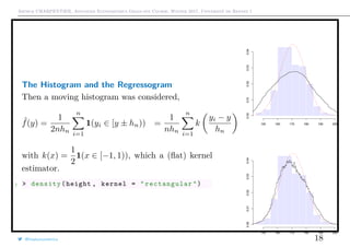
The Histogram and the Regressogram
Connections between the estimation of f(y) and E[Y |X = x].
Assume that yi ∈ [a1, ak+1), divided in k classes [aj, aj+1). The histogram is
ˆfa(y) =
k
j=1
1(t ∈ [aj, aj+1))
aj+1 − aj
1
n
n
i=1
1(yi ∈ [aj, aj+1))
Assume that aj+1 −aj = hn and hn → 0 as n → ∞
with nhn → ∞ then
E ( ˆfa(y) − f(y))2
∼ O(n−2/3
)
(for an optimal choice of hn).
1 > hist(height)
@freakonometrics 17
150 160 170 180 190
0.000.010.020.030.040.050.06](https://image.slidesharecdn.com/slides-econometrics-2017-graduate-1-170209234511/85/Econometrics-PhD-Course-1-Nonlinearities-17-320.jpg)
![Arthur CHARPENTIER, Advanced Econometrics Graduate Course, Winter 2017, Université de Rennes 1
The Histogram and the Regressogram
From Tukey (1961) Curves as parameters, and touch
estimation, the regressogram is defined as
ˆma(x) =
n
i=1 1(xi ∈ [aj, aj+1))yi
n
i=1 1(xi ∈ [aj, aj+1))
and the moving regressogram is
ˆm(x) =
n
i=1 1(xi ∈ [x ± hn])yi
n
i=1 1(xi ∈ [x ± hn])
@freakonometrics 19
q
q
q
q
q
q
q
q
q
q
q
q
q
q
q
q
qq
q
q
q
q
q
q
q
q
q
q
q
q
q
q
q
q
q
q
q
q
q
q
q
q
q
q
q
q
qq
q
q
5 10 15 20 25
020406080100120
speed
dist
q
q
q
q
q
q
q
q
q
q
q
q
q
q
q
q
qq
q
q
q
q
q
q
q
q
q
q
q
q
q
q
q
q
q
q
q
q
q
q
q
q
q
q
q
q
qq
q
q
5 10 15 20 25
020406080100120
speed
dist](https://image.slidesharecdn.com/slides-econometrics-2017-graduate-1-170209234511/85/Econometrics-PhD-Course-1-Nonlinearities-19-320.jpg)
![Arthur CHARPENTIER, Advanced Econometrics Graduate Course, Winter 2017, Université de Rennes 1
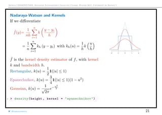
Nadaraya-Watson and Kernels
Background: Kernel Density Estimator
Consider sample {y1, · · · , yn}, Fn empirical cumulative distribution function
Fn(y) =
1
n
n
i=1
1(yi ≤ y)
The empirical measure Pn consists in weights 1/n on each observation.
Idea: add (little) continuous noise to smooth Fn.
Let Yn denote a random variable with distribution Fn and define
˜Y = Yn + hU where U ⊥⊥ Yn, with cdf K
The cumulative distribution function of ˜Y is ˜F
˜F(y) = P[ ˜Y ≤ y] = E 1( ˜Y ≤ y) = E E 1( ˜Y ≤ y) Yn
˜F(y) = E 1 U ≤
y − Yn
h
Yn =
n
i=1
1
n
K
y − yi
h
@freakonometrics 20](https://image.slidesharecdn.com/slides-econometrics-2017-graduate-1-170209234511/85/Econometrics-PhD-Course-1-Nonlinearities-20-320.jpg)
![Arthur CHARPENTIER, Advanced Econometrics Graduate Course, Winter 2017, Université de Rennes 1
Kernels and Statistical Properties
Consider here an i.id. sample {Y1, · · · , Yn} with density f
Given y, observe that E[ ˜f(y)] =
1
h
k
y − t
h
f(t)dt = k(u)f(y − hu)du. Use
Taylor expansion around h = 0,f(y − hu) ∼ f(y) − f (y)hu +
1
2
f (y)h2
u2
E[ ˜f(y)] = f(y)k(u)du − f (y)huk(u)du +
1
2
f (y + hu)h2
u2
k(u)du
= f(y) + 0 + h2 f (y)
2
k(u)u2
du + o(h2
)
Thus, if f is twice continuously differentiable with bounded second derivative,
k(u)du = 1, uk(u)du = 0 and u2
k(u)du < ∞,
then E[ ˜f(y)] = f(y) + h2 f (y)
2
k(u)u2
du + o(h2
)
@freakonometrics 22](https://image.slidesharecdn.com/slides-econometrics-2017-graduate-1-170209234511/85/Econometrics-PhD-Course-1-Nonlinearities-22-320.jpg)
![Arthur CHARPENTIER, Advanced Econometrics Graduate Course, Winter 2017, Université de Rennes 1
Kernels and Statistical Properties
For the heuristics on that bias, consider a flat kernel,
and set
fh(y) =
F(y + h) − F(y − h)
2h
then the natural estimate is
fh(y) =
F(y + h) − F(y − h)
2h
=
1
2nh
n
i=1
1(yi ∈ [y ± h])
Zi
where Zi’s are Bernoulli B(px) i.id. variables with
px = P[Yi ∈ [x ± h]] = 2h · fh(x). Thus, E(fh(y)) = fh(y), while
fh(y) ∼ f(y) +
h2
6
f (y) as h ∼ 0.
@freakonometrics 23](https://image.slidesharecdn.com/slides-econometrics-2017-graduate-1-170209234511/85/Econometrics-PhD-Course-1-Nonlinearities-23-320.jpg)
![Arthur CHARPENTIER, Advanced Econometrics Graduate Course, Winter 2017, Université de Rennes 1
Kernels and Statistical Properties
Similarly, as h → 0 and nh → ∞
Var[ ˜f(y)] =
1
n
E[kh(z − Z)2
] − (E[kh(z − Z)])
2
Var[ ˜f(y)] =
f(y)
nh
k(u)2
du + o
1
nh
Hence
• if h → 0 the bias goes to 0
• if nh → ∞ the variance goes to 0
@freakonometrics 24](https://image.slidesharecdn.com/slides-econometrics-2017-graduate-1-170209234511/85/Econometrics-PhD-Course-1-Nonlinearities-24-320.jpg)
![Arthur CHARPENTIER, Advanced Econometrics Graduate Course, Winter 2017, Université de Rennes 1
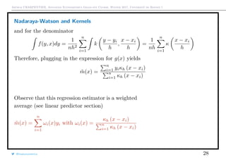
Nadaraya-Watson and Kernels
Here E[Y |X = x] = m(x). Write m as a function of densities
g(x) = yf(y|x)dy =
yf(y, x)dy
f(y, x)dy
Consider some bivariate kernel k, such that
tk(t, u)dt = 0 and κ(u) = k(t, u)dt
For the numerator, it can be estimated using
y ˜f(y, x)dy =
1
nh2
n
i=1
yk
y − yi
h
,
x − xi
h
=
1
nh
n
i=1
yik t,
x − xi
h
dt =
1
nh
n
i=1
yiκ
x − xi
h
@freakonometrics 27](https://image.slidesharecdn.com/slides-econometrics-2017-graduate-1-170209234511/85/Econometrics-PhD-Course-1-Nonlinearities-27-320.jpg)
![Arthur CHARPENTIER, Advanced Econometrics Graduate Course, Winter 2017, Université de Rennes 1
Nadaraya-Watson and Kernels
One can prove that kernel regression bias is given by
E[ ˜m(x)] = m(x) + C1h2 1
2
m (x) + m (x)
f (x)
f(x)
In the univariate case, one can get the kernel estimator of derivatives
d ˜m(x)
dx
=
1
nh2
n
i=1
k
x − xi
h
yi
Actually, ˜m is a function of bandwidth h.
Note: this can be extended to multivariate x.
@freakonometrics 29
q
q
q
q
q
q
q
q
q
q
q
q
q
q
q
q
qq
q
q
q
q
q
q
q
q
q
q
q
q
q
q
q
q
q
q
q
q
q
q
q
q
q
q
q
q
qq
q
q
5 10 15 20 25
020406080100120
speed
dist
q](https://image.slidesharecdn.com/slides-econometrics-2017-graduate-1-170209234511/85/Econometrics-PhD-Course-1-Nonlinearities-29-320.jpg)
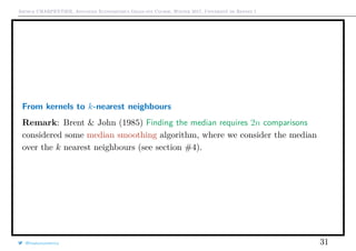
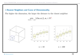
![Arthur CHARPENTIER, Advanced Econometrics Graduate Course, Winter 2017, Université de Rennes 1
From kernels to k-nearest neighbours
An alternative is to consider
˜mk(x) =
1
n
n
i=1
ωi,k(x)yi
where ωi,k(x) =
n
k
if i ∈ Ik
x with
Ik
x = {i : xi one of the k nearest observations to x}
Lai (1977) Large sample properties of K-nearest neighbor procedures if k → ∞ and
k/n → 0 as n → ∞, then
E[ ˜mk(x)] ∼ m(x) +
1
24f(x)3
(m f + 2m f )(x)
k
n
2
while Var[ ˜mk(x)] ∼
σ2
(x)
k
@freakonometrics 30
q
q
q
q
q
q
q
q
q
q
q
q
q
q
q
q
qq
q
q
q
q
q
q
q
q
q
q
q
q
q
q
q
q
q
q
q
q
q
q
q
q
q
q
q
q
qq
q
q
5 10 15 20 25
020406080100120
speed
dist](https://image.slidesharecdn.com/slides-econometrics-2017-graduate-1-170209234511/85/Econometrics-PhD-Course-1-Nonlinearities-30-320.jpg)
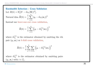
![Arthur CHARPENTIER, Advanced Econometrics Graduate Course, Winter 2017, Université de Rennes 1
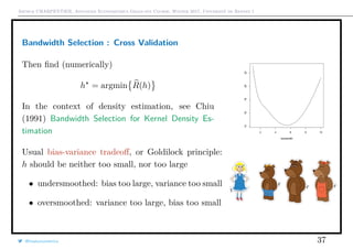
Bandwidth selection : MISE for Density
MSE[ ˜f(y)] = bias[ ˜f(y)]2
+ Var[ ˜f(y)]
MSE[ ˜f(y)] = f(y)
1
nh
k(u)2
du + h4 f (y)
2
k(u)u2
du
2
+ o h4
+
1
nh
Bandwidth choice is based on minimization of the asymptotic integrated MSE
(over y)
MISE( ˜f) = MSE[ ˜f(y)]dy ∼
1
nh
k(u)2
du + h4 f (y)
2
k(u)u2
du
2
@freakonometrics 33](https://image.slidesharecdn.com/slides-econometrics-2017-graduate-1-170209234511/85/Econometrics-PhD-Course-1-Nonlinearities-33-320.jpg)
![Arthur CHARPENTIER, Advanced Econometrics Graduate Course, Winter 2017, Université de Rennes 1
Bandwidth selection : MISE for Density
Thus, the first-order condition yields
−
C1
nh2
+ h3
f (y)2
dyC2 = 0
with C1 = k2
(u)du and C2 = k(u)u2
du
2
, and
h = n− 1
5
C1
C2 f (y)dy
1
5
h = 1.06n− 1
5 Var[Y ] from Silverman (1986) Density Estimation
1 > bw.nrd0(cars$speed)
2 [1] 2.150016
3 > bw.nrd(cars$speed)
4 [1] 2.532241
with Scott correction, see Scott (1992) Multivariate Density Estimation
@freakonometrics 34](https://image.slidesharecdn.com/slides-econometrics-2017-graduate-1-170209234511/85/Econometrics-PhD-Course-1-Nonlinearities-34-320.jpg)
![Arthur CHARPENTIER, Advanced Econometrics Graduate Course, Winter 2017, Université de Rennes 1
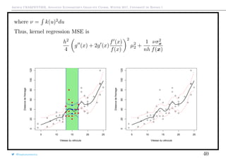
Bandwidth selection : MISE for Regression Model
One can prove that
MISE[mh] ∼
bias2
h4
4
x2
k(x)dx
2
m (x) + 2m (x)
f (x)
f(x)
2
dx
+
σ2
nh
k2
(x)dx ·
dx
f(x)
variance
as n → 0 and nh → ∞.
The bias is sensitive to the position of the xi’s.
h = n− 1
5
C1
dx
f(x)
C2 m (x) + 2m (x)f (x)
f(x) dx
1
5
Problem: depends on unknown f(x) and m(x).
@freakonometrics 35](https://image.slidesharecdn.com/slides-econometrics-2017-graduate-1-170209234511/85/Econometrics-PhD-Course-1-Nonlinearities-35-320.jpg)
![Arthur CHARPENTIER, Advanced Econometrics Graduate Course, Winter 2017, Université de Rennes 1
Local Linear Regression
Consider ˆm(x) defined as ˆm(x) = β0 where (β0, β) is the solution of
min
(β0,β)
n
i=1
ω
(x)
i yi − [β0 + (x − xi)T
β]
2
where ω
(x)
i = kh(x − xi), e.g.
i.e. we seek the constant term in a weighted least squares regression of yi’s on
x − xi’s. If Xx is the matrix [1 (x − X)T
], and if W x is a matrix
diag[kh(x − x1), · · · , kh(x − xn)]
then ˆm(x) = 1T
(XT
xW xXx)−1
XT
xW xy
This estimator is also a linear predictor :
ˆm(x) =
n
i=1
ai(x)
ai(x)
yi
@freakonometrics 38](https://image.slidesharecdn.com/slides-econometrics-2017-graduate-1-170209234511/85/Econometrics-PhD-Course-1-Nonlinearities-38-320.jpg)
![Arthur CHARPENTIER, Advanced Econometrics Graduate Course, Winter 2017, Université de Rennes 1
where
ai(x) =
1
n
kh(x − xi) 1 − s1(x)T
s2(x)−1 x − xi
h
with
s1(x) =
1
n
n
i=1
kh(x−xi)
x − xi
h
and s2(x) =
1
n
n
i=1
kh(x−xi)
x − xi
h
x − xi
h
Note that Nadaraya-Watson estimator was simply the solution of
min
β0
n
i=1
ω
(x)
i (yi − β0)
2
where ω
(x)
i = kh(x − xi)
E[ ˆm(x)] ∼ m(x) +
h2
2
m (x)µ2 where µ2 = k(u)u2
du.
Var[ ˆm(x)] ∼
1
nh
νσ2
x
f(x)
@freakonometrics 39](https://image.slidesharecdn.com/slides-econometrics-2017-graduate-1-170209234511/85/Econometrics-PhD-Course-1-Nonlinearities-39-320.jpg)
![Arthur CHARPENTIER, Advanced Econometrics Graduate Course, Winter 2017, Université de Rennes 1
Local polynomials
One might assume that, locally, m(x) ∼ µx(u) as u ∼ 0, with
µx(u) = β
(x)
0 + β
(x)
1 + [u − x] + β
(x)
2 +
[u − x]2
2
+ β
(x)
3 +
[u − x]3
2
+ · · ·
and we estimate β(x)
by minimizing
n
i=1
ω
(x)
i yi − µx(xi)
2
.
If Xx is the design matrix 1 xi − x
[xi − x]2
2
[xi − x]3
3
· · · , then
β
(x)
= XT
xW xXx
−1
XT
xW xy
(weighted least squares estimators).
1 > library(locfit)
2 > locfit(dist~speed ,data=cars)
@freakonometrics 42](https://image.slidesharecdn.com/slides-econometrics-2017-graduate-1-170209234511/85/Econometrics-PhD-Course-1-Nonlinearities-42-320.jpg)
![Arthur CHARPENTIER, Advanced Econometrics Graduate Course, Winter 2017, Université de Rennes 1
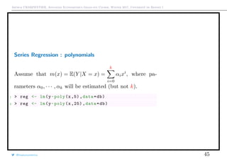
Series Regression
Recall that E[Y |X = x] = m(x).
Why not approximate m by a linear combination of approx-
imating functions h1(x), · · · , hk(x).
Set h(x) = (h1(x), · · · , hk(x)), and consider the regression
of yi’s on h(xi)’s,
yi = h(xi)T
β + εi
Then β = (HT
H)−1
HT
y
q
q
q
q
q
q
q
q
q
q
q
q
q
q
q
q
qq
q
q
q
q
q
q
q
q
q
q
q
q
q
q
q
q
q
q
q
q
q
q
q
q
q
q
q
q
qq
q
q
5 10 15 20 25
020406080100120
Vitesse du véhciule
Distancedefreinage
q
q
q
q
q
q
q
q
q
q
q
q
q
q
q
q
qq
q
q
q
q
q
q
q
q
q
q
q
q
q
q
q
q
q
q
q
q
q
q
q
q
q
q
q
q
qq
q
q
q
q
q
q
q
q
q
q
q
q
q
q
q
q
q
q
q
q
q
q
q
q
q
q
q
q
q
q
q
q
q
q
q
q
q
q
q
q
q
q
q
q
q
qq
q
q
q
q
q
q
q
q
q
q
q
q
q
q
q
q
q
q
q
q
q
q
q
q
q
q
q
q
qq
q
q
5 10 15 20 25
020406080100120
Vitesse du véhciule
Distancedefreinage
@freakonometrics 43](https://image.slidesharecdn.com/slides-econometrics-2017-graduate-1-170209234511/85/Econometrics-PhD-Course-1-Nonlinearities-43-320.jpg)
![Arthur CHARPENTIER, Advanced Econometrics Graduate Course, Winter 2017, Université de Rennes 1
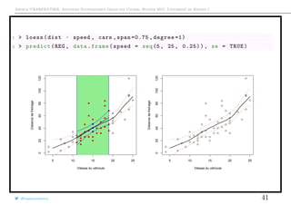
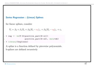
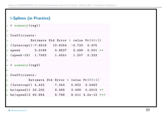
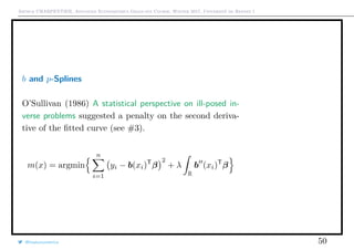
b-Splines (in Practice)
1 > reg1 <- lm(dist~speed+positive_part(speed -15) ,
data=cars)
2 > reg2 <- lm(dist~bs(speed ,df=2, degree =1) , data=
cars)
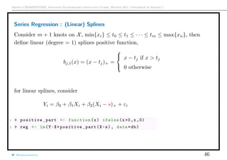
Consider m+1 knots on [0, 1], 0 ≤ t0 ≤ t1 ≤ · · · ≤ tm ≤ 1,
then define recursively b-splines as
bj,0(t) =
1 if tj ≤ t < tj+1
0 otherwise, and
bj,n(t) =
t − tj
tj+n − tj
bj,n−1(t)
+
tj+n+1 − t
tj+n+1 − tj+1
bj+1,n−1(t)
q
q
q
q
q
q
q
q
q
q
q
q
q
q
q
q
qq
q
q
q
q
q
q
q
q
q
q
q
q
q
q
q
q
q
q
q
q
q
q
q
q
q
q
q
q
qq
q
q
5 10 15 20 25
020406080100120
speed
dist
q
q
q
q
q
q
q
q
q
q
q
q
q
q
q
q
qq
q
q
q
q
q
q
q
q
q
q
q
q
q
q
q
q
q
q
q
q
q
q
q
q
q
q
q
q
qq
q
q
5 10 15 20 25
020406080100120
speed
dist
@freakonometrics 48](https://image.slidesharecdn.com/slides-econometrics-2017-graduate-1-170209234511/85/Econometrics-PhD-Course-1-Nonlinearities-48-320.jpg)
![Arthur CHARPENTIER, Advanced Econometrics Graduate Course, Winter 2017, Université de Rennes 1
Adding Constraints: Convex Regression
Assume that yi = m(xi) + εi where m : Rd
→ ∞R is some convex function.
m is convex if and only if ∀x1, x2 ∈ Rd
, ∀t ∈ [0, 1],
m(tx1 + [1 − t]x2) ≤ tm(x1) + [1 − t]m(x2)
Proposition (Hidreth (1954) Point Estimates of Ordinates of Concave Functions)
m = argmin
m convex
n
i=1
yi − m(xi)
2
Then θ = (m (x1), · · · , m (xn)) is unique.
Let y = θ + ε, then
θ = argmin
θ∈K
n
i=1
yi − θi)
2
where K = {θ ∈ Rn
: ∃m convex , m(xi) = θi}. I.e. θ is the projection of y onto
the (closed) convex cone K. The projection theorem gives existence and unicity.
@freakonometrics 51](https://image.slidesharecdn.com/slides-econometrics-2017-graduate-1-170209234511/85/Econometrics-PhD-Course-1-Nonlinearities-51-320.jpg)
![Arthur CHARPENTIER, Advanced Econometrics Graduate Course, Winter 2017, Université de Rennes 1
Adding Constraints: Convex Regression
In dimension 1: yi = m(xi) + εi. Assume that observations are ordered
x1 < x2 < · · · < xn.
Here
K = θ ∈ Rn
:
θ2 − θ1
x2 − x1
≤
θ3 − θ2
x3 − x2
≤ · · · ≤
θn − θn−1
xn − xn−1
Hence, quadratic program with n − 2 linear con-
straints.
m is a piecewise linear function (interpolation of
consecutive pairs (xi, θi )).
If m is differentiable, m is convex if
m(x) + m(x) · [y − x] ≤ m(y)
q
q
q
q
q
q
q
q
q
q
q
q
q
q
q
q
qq
q
q
q
q
q
q
q
q
q
q
q
q
q
q
q
q
q
q
q
q
q
q
q
q
q
q
q
q
qq
q
q
5 10 15 20 25
020406080100120
speed
dist
@freakonometrics 52](https://image.slidesharecdn.com/slides-econometrics-2017-graduate-1-170209234511/85/Econometrics-PhD-Course-1-Nonlinearities-52-320.jpg)
![Arthur CHARPENTIER, Advanced Econometrics Graduate Course, Winter 2017, Université de Rennes 1
Adding Constraints: Convex Regression
More generally: if m is convex, then there exists ξx ∈ Rn
such that
m(x) + ξx · [y − x] ≤ m(y)
ξx is a subgradient of m at x. And then
∂m(x) = m(x) + ξ · [y − x] ≤ m(y), ∀y ∈ Rn
Hence, θ is solution of
argmin y − θ 2
subject to θi + ξi[xj − xi] ≤ θj, ∀i, j
and ξ1, · · · , ξn ∈ Rn
.
@freakonometrics 53
q
q
q
q
q
q
q
q
q
q
q
q
q
q
q
q
qq
q
q
q
q
q
q
q
q
q
q
q
q
q
q
q
q
q
q
q
q
q
q
q
q
q
q
q
q
qq
q
q
5 10 15 20 25
020406080100120
speed
dist](https://image.slidesharecdn.com/slides-econometrics-2017-graduate-1-170209234511/85/Econometrics-PhD-Course-1-Nonlinearities-53-320.jpg)
![Arthur CHARPENTIER, Advanced Econometrics Graduate Course, Winter 2017, Université de Rennes 1
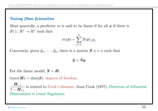
Testing (Non-)Linearities
In the linear model,
y = Xβ = X[XT
X]−1
XT
H
y
Hi,i is the leverage of the ith element of this hat matrix.
Write
yi =
n
j=1
[XT
i [XT
X]−1
XT
]jyj =
n
j=1
[H(Xi)]jyj
where
H(x) = xT
[XT
X]−1
XT
The prediction is
m(x) = E(Y |X = x) =
n
j=1
[H(x)]jyj
@freakonometrics 54](https://image.slidesharecdn.com/slides-econometrics-2017-graduate-1-170209234511/85/Econometrics-PhD-Course-1-Nonlinearities-54-320.jpg)
![Arthur CHARPENTIER, Advanced Econometrics Graduate Course, Winter 2017, Université de Rennes 1
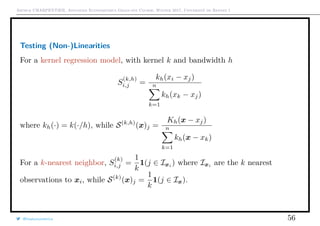
Testing (Non-)Linearities
Observe that trace(S) is usually seen as a degree of smoothness.
Do we have to smooth? Isn’t linear model sufficent?
Define
T =
Sy − Hy
trace([S − H]T[S − H])
If the model is linear, then T has a Fisher distribution.
Remark: In the case of a linear predictor, with smoothing matrix Sh
R(h) =
1
n
n
i=1
(yi − m
(−i)
h (xi))2
=
1
n
n
i=1
Yi − mh(xi)
1 − [Sh]i,i
2
We do not need to estimate n models.
@freakonometrics 57](https://image.slidesharecdn.com/slides-econometrics-2017-graduate-1-170209234511/85/Econometrics-PhD-Course-1-Nonlinearities-57-320.jpg)
![Arthur CHARPENTIER, Advanced Econometrics Graduate Course, Winter 2017, Université de Rennes 1
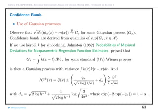
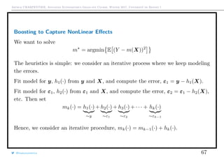
Boosting
h(x) = y − mk(x), which can be interpreted as a residual. Note that this residual
is the gradient of
1
2
[y − mk(x)]2
A gradient descent is based on Taylor expansion
f(xk)
f,xk
∼ f(xk−1)
f,xk−1
+ (xk − xk−1)
α
f(xk−1)
f,xk−1
But here, it is different. We claim we can write
fk(x)
fk,x
∼ fk−1(x)
fk−1,x
+ (fk − fk−1)
β
?
fk−1, x
where ? is interpreted as a ‘gradient’.
@freakonometrics 68](https://image.slidesharecdn.com/slides-econometrics-2017-graduate-1-170209234511/85/Econometrics-PhD-Course-1-Nonlinearities-68-320.jpg)
![Arthur CHARPENTIER, Advanced Econometrics Graduate Course, Winter 2017, Université de Rennes 1
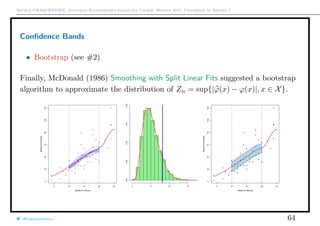
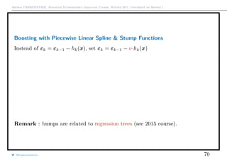
Boosting
Here, fk is a Rd
→ R function, so the gradient should be in such a (big)
functional space → want to approximate that function.
mk(x) = mk−1(x) + argmin
f∈F
n
i=1
(yi − [mk−1(x) + f(x)])2
where f ∈ F means that we seek in a class of weak learner functions.
If learner are two strong, the first loop leads to some fixed point, and there is no
learning procedure, see linear regression y = xT
β + ε. Since ε ⊥ x we cannot
learn from the residuals.
In order to make sure that we learn weakly, we can use some shrinkage
parameter ν (or collection of parameters νj).
@freakonometrics 69](https://image.slidesharecdn.com/slides-econometrics-2017-graduate-1-170209234511/85/Econometrics-PhD-Course-1-Nonlinearities-69-320.jpg)
![Arthur CHARPENTIER, Advanced Econometrics Graduate Course, Winter 2017, Université de Rennes 1
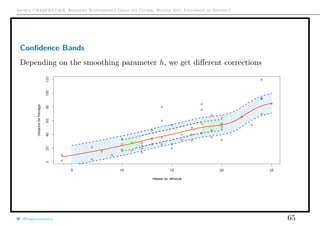
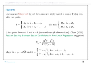
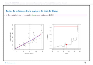
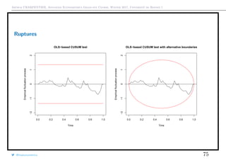
Ruptures
If i0 is unknown, use CUSUM types of tests, see Ploberger & Krämer (1992) The
Cusum Test with OLS Residuals. For all t ∈ [0, 1], set
Wt =
1
σ
√
n
nt
i=1
εi.
If α is the confidence level, bounds are generally ±α, even if theoretical bounds
should be ±α t(1 − t).
1 > cusum <- efp(dist ~ speed , type = "OLS -CUSUM",data=cars)
2 > plot(cusum ,ylim=c(-2,2))
3 > plot(cusum , alpha = 0.05 , alt.boundary = TRUE ,ylim=c(-2,2))
@freakonometrics 74](https://image.slidesharecdn.com/slides-econometrics-2017-graduate-1-170209234511/85/Econometrics-PhD-Course-1-Nonlinearities-74-320.jpg)
![Arthur CHARPENTIER, Advanced Econometrics Graduate Course, Winter 2017, Université de Rennes 1
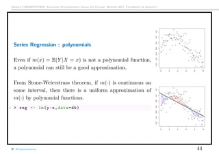
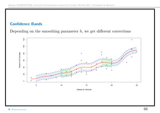
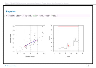
Generalized Additive Models
Linear regression model E[Y |X = x] = β0 + xT
β = β0 +
p
j=1
βjxj
Additive model E[Y |X = x] = β0 +
p
j=1
hj(xj) where hj(·) can be any nonlinear
function.
1 > library(mgcv)
2 > gam(dist~s(speed),
data=cars)
@freakonometrics 77
0.0 0.2 0.4 0.6 0.8 1.0
0.0
0.2
0.4
0.6
0.8
1.0
−0.5
0.0
0.5
1.0
1.5
0.0 0.2 0.4 0.6 0.8 1.0
0.0
0.2
0.4
0.6
0.8
1.0
−0.5
0.0
0.5
1.0
1.5](https://image.slidesharecdn.com/slides-econometrics-2017-graduate-1-170209234511/85/Econometrics-PhD-Course-1-Nonlinearities-77-320.jpg)

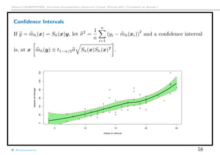
This document is an excerpt from a graduate course on advanced econometrics taught by Arthur Charpentier at Université de Rennes 1 in winter 2017. It discusses the origins and meaning of the term "regression" as coined by Francis Galton in reference to the tendency of offspring to regress towards the mean traits of the general population from their parents' traits. It also includes R code and plots demonstrating this concept using Galton's data on parental and offspring height.