Downloaded 17 times


![Arthur CHARPENTIER - Sales forecasting.
Dening stationarity
Time series (Xt) is weakly stationary if
for all t, E X2
t +∞,
for all t, E (Xt) = µ, constant independent of t,
for all t and for all h, cov (Xt, Xt+h) = E ([Xt − µ] [Xt+h − µ]) = γ (h),
independent of t.
Function γ (·) is called autocovariance function.
Given a stationary series (Xt) , dene the autocovariance function, as
h → γX (h) = cov (Xt, Xt−h) = E (XtXt−h) − E (Xt) .E (Xt−h) .
and dene the autocorrelation function, as
h → ρX (h) = corr (Xt, Xt−h) =
cov (Xt, Xt−h)
V (Xt) V (Xt−h)
=
γX (h)
γX (0)
.
26](https://image.slidesharecdn.com/slides-sales-forecasting-session2-web-130711204206-phpapp02/85/Slides-sales-forecasting-session2-web-26-320.jpg)


![Arthur CHARPENTIER - Sales forecasting.
Geometry and probability
Recall that it is possible to dene an inner product in L2
(space of squared
integrable variables, i.e. nite variance),
X, Y = E ([X − E(X)] · [Y − E(Y )]) = cov([X − E(X)], [Y − E(Y )])
Then the associated norm is ||X||2
= E [X − E(X)]2
= V (X).
Two random variables are then orthogonal if X, Y = 0, i.e.
cov([X − E(X)], [Y − E(Y )]) = 0.
Hence conditional expectation is simply a projection in the L2
, E(X|Y ) is the the
projection is the space generated by Y of random variable X, i.e.
E(X|Y ) = φ(Y ), such that
X − φ(Y ) ⊥ X, i.e. X − φ(Y ), X = 0,
φ(Y ) = Z∗
= argmin{Z = h(Y ), ||X − Z||2
}
E(φ(Y )) ∞.
32](https://image.slidesharecdn.com/slides-sales-forecasting-session2-web-130711204206-phpapp02/85/Slides-sales-forecasting-session2-web-32-320.jpg)


![Arthur CHARPENTIER - Sales forecasting.
Moving average process MA(q)
We call moving average process of order q, denoted MA (q), a stationnary
process (Xt) satisfying equation
Xt = εt +
q
i=1
θiεt−i for all t ∈ Z, (3)
where the θi's are real-valued coecients, and process (εt) is a white noise
process with variance σ2
. (3) processes can be written equivalently
Xt = Θ (L) εt whereΘ (L) = I + θ1L + ... + θqLq
.
The autocovariance function satises
γ (h) = E (XtXt−h)
= E ([εt + θ1εt−1 + ... + θqεt−q] [εt−h + θ1εt−h−1 + ... + θqεt−h−q])
=
[θh + θh+1θ1 + ... + θqθq−h] σ2
if 1 ≤ h ≤ q
0 if h q,
65](https://image.slidesharecdn.com/slides-sales-forecasting-session2-web-130711204206-phpapp02/85/Slides-sales-forecasting-session2-web-65-320.jpg)


![Arthur CHARPENTIER - Sales forecasting.
Forecasting with AR(1) processes
Consider an AR (1) process, Xt = µ + φXt−1 + εt then
• T X∗
T +1 = µ + φXT ,
• T X∗
T +2 = µ + φ.T X∗
T +1 = µ + φ [µ + φXT ] = µ [1 + φ] + φ2
XT ,
• T X∗
T +3 = µ + φ.T X∗
T +2 = µ + φ [µ + φ [µ + φXT ]] = µ 1 + φ + φ2
+ φ3
XT ,
and recursively T X∗
T +h can be written
T X∗
T +h = µ + φ.T X∗
T +h−1 = µ 1 + φ + φ2
+ ... + φh−1
+ φh
XT .
or equivalently
T X∗
T +h =
µ
φ
+ φh
XT −
µ
φ
= µ
1 − φh
1 − φ
1+φ+φ2+...+φh−1
+ φh
XT .
75](https://image.slidesharecdn.com/slides-sales-forecasting-session2-web-130711204206-phpapp02/85/Slides-sales-forecasting-session2-web-75-320.jpg)
![Arthur CHARPENTIER - Sales forecasting.
Forecasting with AR(1) processes
The forecasting error made at time T for horizon h is
T ∆h = T X∗
T +h − XT +h =T X∗
T +h − [φXT +h−1 + µ + εT +h]
= ...
= T X∗
T +h − φh
1 XT + φh−1
+ ... + φ + 1 µ
+εT +h + φεT +h−1 + ... + φh−1
εT +1,
(6)
thus, T ∆h = εT +h + φεT +h−1 + ... + φh−1
εT +1, with variance having variance
V = 1 + φ2
+ φ4
+ ... + φ2h−2
σ2
, where V (εt) = σ2
.
thus, variance of the forecast error increasing with horizon.
76](https://image.slidesharecdn.com/slides-sales-forecasting-session2-web-130711204206-phpapp02/85/Slides-sales-forecasting-session2-web-76-320.jpg)

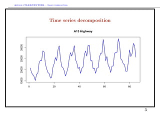
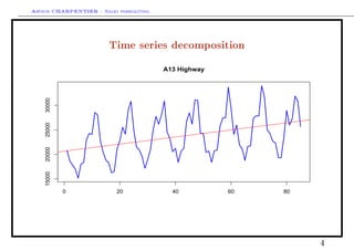
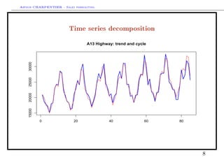
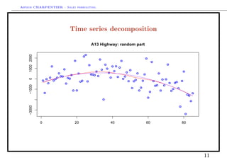
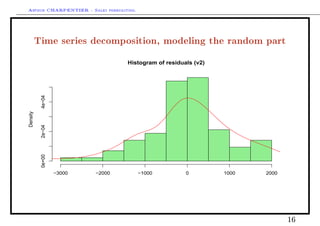
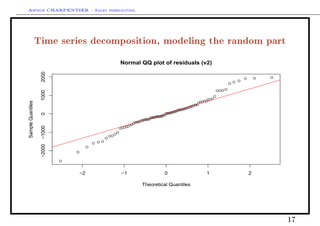
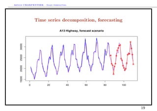
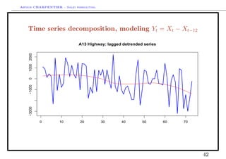
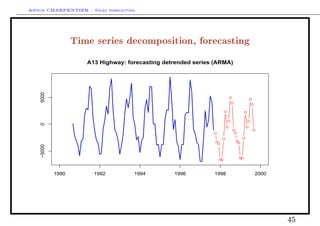
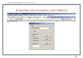
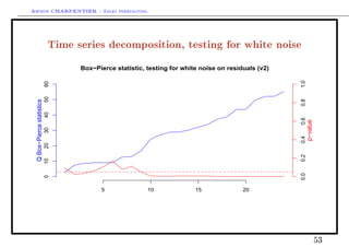
This document discusses time series decomposition and forecasting methods. It begins with an overview of qualitative and quantitative forecasting techniques, including short and long term forecasting and regression methods. It then focuses on Box-Jenkins ARIMA time series modeling, demonstrating decomposition of a time series into trend, seasonal, and random components. Forecasting involves modeling these components and generating predictions. Practical issues with forecasting in Excel are also mentioned. Overall the document provides an introduction to time series analysis and forecasting techniques.