Download as PDF, PPTX


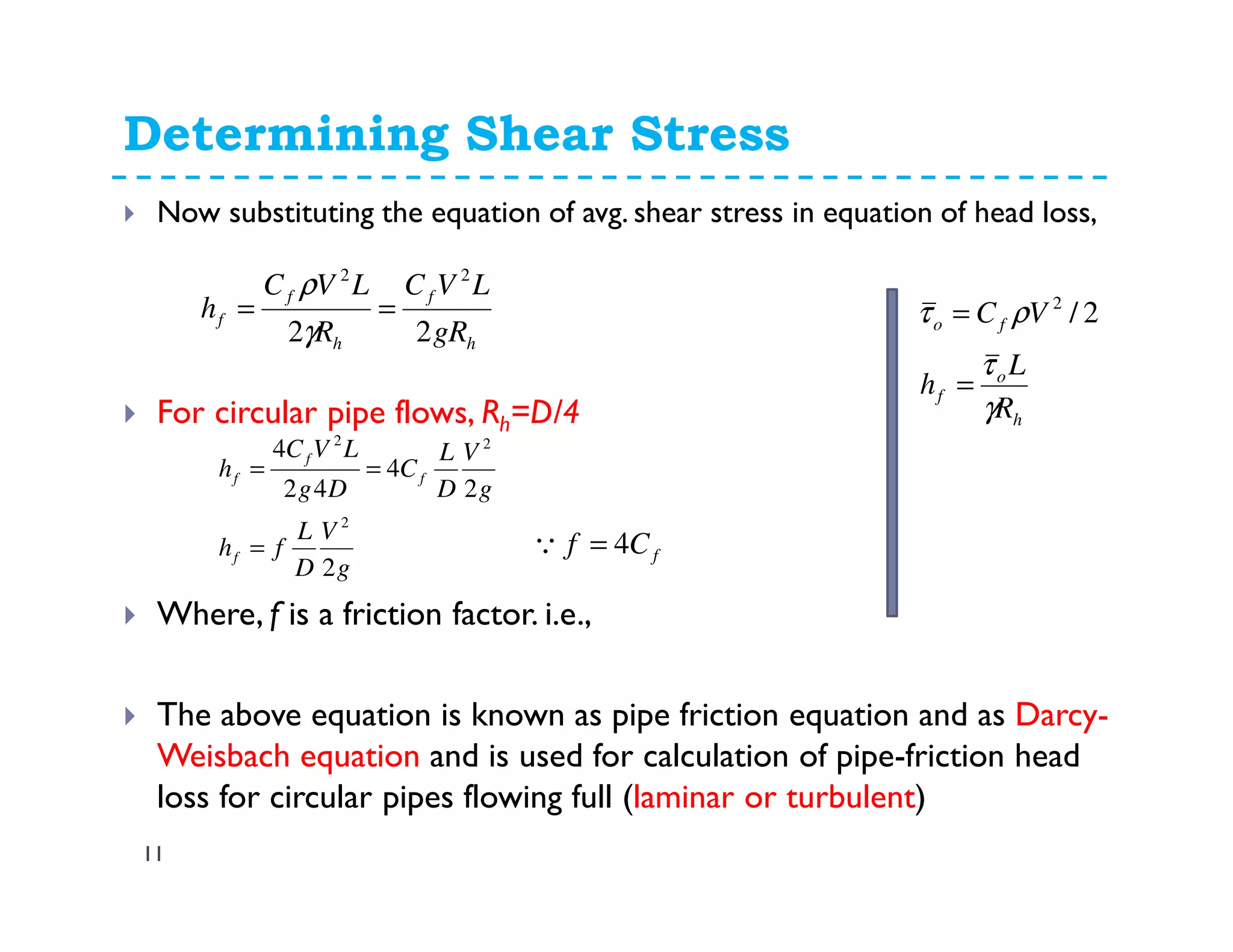


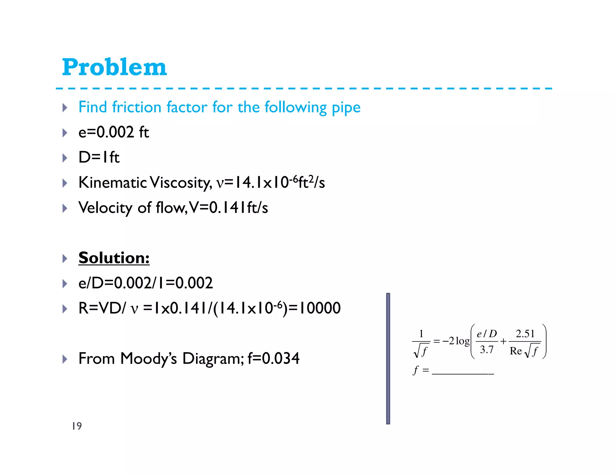


1. Given: Pipe characteristics (D, L, e), fluid properties (ν), flow conditions (Q or V) 2. Calculate Reynold's number (Re) using the given flow parameters 3. Determine friction factor (f) from Moody diagram or equations based on Re and relative roughness (e/D) 4. Use Darcy-Weisbach equation to calculate head loss (hf) or solve for unknown parameter (Q or V)


![Geotechnical Engineering-I [Lec #27: Flow Nets]](https://cdn.slidesharecdn.com/ss_thumbnails/27-180924141458-thumbnail.jpg?width=640&height=640&fit=bounds)


![Engineering Economics: Solved exam problems [ch1-ch4]](https://cdn.slidesharecdn.com/ss_thumbnails/solvedexamproblemsch1-ch4-200220070043-thumbnail.jpg?width=640&height=640&fit=bounds)