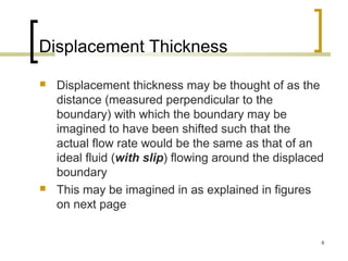
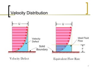
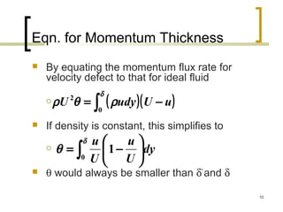
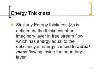
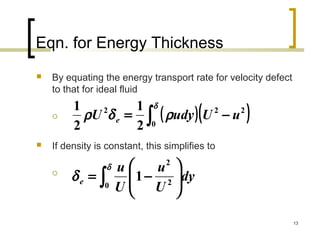
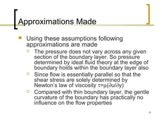
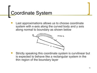
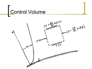
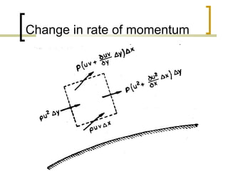
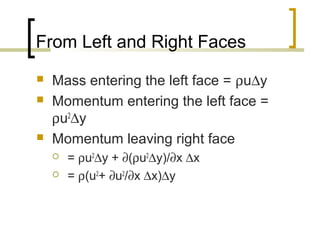
1) The document discusses different definitions of boundary layer thickness, including nominal thickness, displacement thickness, momentum thickness, and energy thickness. Equations are provided for calculating each type of thickness. 2) Key assumptions of boundary layer theory are that the boundary layer is thin compared to the body and flow is two-dimensional and steady. The Prandtl boundary layer equations are derived using control volume analysis and assumptions of constant density and viscosity. 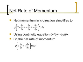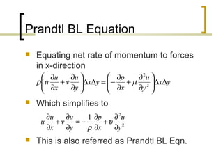3) The Prandtl boundary layer equation equates forces within the boundary layer, including pressure and shear stress, to the net rate of momentum change and forms the basis for boundary layer analysis.

1. Boundary Layer Equations
Prof. Rohit Goyal
Professor, Department of Civil Engineering
Malaviya National Institute of Technology Jaipur
E-Mail: rgoyal_jp@yahoo.com

2. 2
Topics Covered
 Different Boundary Layer Thickness
 Nominal Thickness
 Displacement Thickness
 Momentum Thickness
 Energy Thickness
 Equations for different BL thickness
 Boundary Layer Equations
 Assumptions

3. 3
Nominal Thickness (δ)
 Nominal thickness of the boundary layer
is defined as the thickness of zone
extending from solid boundary to a point
where velocity is 99% of the free stream
velocity (U)
 This is arbitrary, especially because
transition from 0 velocity at boundary to
the U outside the boundary takes place
asymptotically.
 It is based on the fact that beyond this
boundary, effect of viscous stresses can
be neglected.

4. 4
Other Definitions of BL Thickness
 Many other definitions of boundary layer
thickness has been introduced at
different times and provide important
concepts based on mathematical
calculations and logic
 These definitions are
 Displacement Thickness (δ*
)
 Momentum Thickness (θ)
 Energy Thickness (δe)

5. 5
Displacement Thickness
 Presence of boundary layer introduces
a retardation to the free stream
velocity in the neighborhood of the
boundary
 This causes a decrease in mass flow
rate due to presence of boundary layer
 A “velocity defect” of (U-u) exists at a
distance y along y axis

6. 6
Displacement Thickness
 Displacement thickness may be thought of as the
distance (measured perpendicular to the
boundary) with which the boundary may be
imagined to have been shifted such that the
actual flow rate would be the same as that of an
ideal fluid (with slip) flowing around the displaced
boundary
 This may be imagined in as explained in figures
on next page

7. 7
Velocity Distribution
U
Solid
Boundary
Equivalent Flow Rate
U
Velocity Defect
Velocity
Defect
δ*
Ideal Fluid
Flow

8. 8
Eqn. for Displacement Thickness
 By equating the flow rate for velocity defect to
flow rate for ideal fluid

 If density is constant, this simplifies to

 δ*
would always be smaller than δ
( )∫ −=
δ
ρδρ
0
*
dyuUU
∫ 





−=
δ
δ
0
*
1 dy
U
u

9. 9
Momentum Thickness
 Retardation of flow within boundary layer
causes a reduction in the momentum flux
too
 So similar to displacement thickness, the
momentum thickness (θ) is defined as
the thickness of an imaginary layer in free
stream flow which has momentum equal
to the deficiency of momentum caused to
actual mass flowing inside the boundary
layer

10. 10
Eqn. for Momentum Thickness
 By equating the momentum flux rate for
velocity defect to that for ideal fluid

 If density is constant, this simplifies to

 θ would always be smaller than δ*
and δ
( )( )∫ −=
δ
ρθρ
0
2
uUudyU
∫ 





−=
δ
θ
0
1 dy
U
u
U
u

11. 11
Graphical Representation

12. 12
Energy Thickness
 Similarly Energy thickness (δe) is
defined as the thickness of an
imaginary layer in free stream flow
which has energy equal to the
deficiency of energy caused to actual
mass flowing inside the boundary
layer

13. 13
Eqn. for Energy Thickness
 By equating the energy transport rate for velocity defect
to that for ideal fluid

 If density is constant, this simplifies to

( )( )∫ −=
δ
ρδρ
0
222
2
1
2
1
uUudyU e
∫ 





−=
δ
δ
0 2
2
1 dy
U
u
U
u
e

14. 14
Boundary Layer Assumptions
 Following assumptions are made for the analysis
of the boundary layer
 It is assumed (also observed to great extend) that
Reynolds number of flows are large and the
thickness of boundary layer are small in
comparison with any characteristic dimension of
the boundary
 The boundary is streamlined so that the flow
pattern and pressures determined by ideal flow
theory are accurate
 It is possible to treat the flow at constant density
and isothermal conditions prevail so that viscosity
is also constant

15. 15
Approximations Made
 Using these assumptions following
approximations are made
 The pressure does not vary across any given
section of the boundary layer. So pressure
determined by ideal fluid theory at the edge of
boundary holds within the boundary layer also
 Since flow is essentially parallel so that the
shear stress are solely determined by
Newton’s law of viscosity τ=µ(∂u/∂y)
 Compared with thin boundary layer, the gentle
curvature of the boundary has practically no
influence on the flow properties

16. 16
Coordinate System
 Last approximations allows us to choose coordinate
system with x-axis along the curved body and y axis
along normal to boundary as shown below
 Strictly speaking this coordinate system is curvilinear but
is expected to behave like a rectangular system in the
thin region of the boundary layer

17. Continuity Equation
 Only steady two dimensional flow
is considered for simplicity
 Continuity Equation in 2D is
 ∂u/∂x+∂v/∂y = 0
 Where u and v are velocity
components in x and y axes

18. Momentum Equation
 Since velocity component in y direction
is negligibly small so momentum
equation is considered only in x
direction
 Considering a small control volume of
sides ∆x and ∆y and thickness in the
third direction as unity is considered as
shown on next page.

19. Control Volume

20. Summation of Forces
 Neglecting component of gravity in x-
direction, only pressure and shear stress as
shown on control volume are considered
 There would be a negative shear stress on
lower face because layer below is trying to
retard the motion of particles within control
volume. Similarly shear stress on top
surface would be positive
xy
y
xyx
x
p
pypFx ∆





∆
∂
∂
++∆−∆





∆
∂
∂
+−∆=∑
τ
ττ

21. Forces in x-Direction
 So total force in x direction
 Using Newton’s law of viscosity
 This would be equal to change in rate of
momentum in x-direction
xy
y
xyx
x
p
pypFx ∆





∆
∂
∂
++∆−∆





∆
∂
∂
+−∆=∑
τ
ττ
yx
y
u
x
p
Fx ∆∆





∂
∂
+
∂
∂
−=∑ 2
2
µ

22. Change in rate of momentum

23. From Left and Right Faces
 Mass entering the left face = ρu∆y
 Momentum entering the left face =
ρu2
∆y
 Momentum leaving right face
 = ρu2
∆y + ∂(ρu2
∆y)/∂x ∆x
 = ρ(u2
+ ∂u2
/∂x ∆x)∆y

24. From Top and Bottom faces
 Mass entering from bottom face = ρv∆x
 Momentum entering the bottom face =
(ρv∆x)u
 Momentum leaving top face
 = ρuv∆x + ∂(ρuv∆x)/∂y ∆y
 = ρ(uv+ ∂(uv)/∂y ∆y)∆x
 Net momentum in x-direction

( ) xuvyuxy
y
uv
uvyx
x
u
u ∆−∆−∆





∆
∂
∂
++∆





∆
∂
∂
+ ρρρρ 2
2
2

25. Net Rate of Momentum
 Net momentum in x-direction simplifies to
 Using continuity equation ∂v/∂y=-∂u/∂x
 So the net rate of momentum
yx
y
u
v
y
v
u
x
u
u ∆∆





∂
∂
+
∂
∂
+
∂
∂
2ρ
yx
y
u
v
x
u
u ∆∆





∂
∂
+
∂
∂
ρ

26. Prandtl BL Equation
 Equating net rate of momentum to forces
in x-direction
 Which simplifies to
 This is also referred as Prandtl BL Eqn.
yx
y
u
x
p
yx
y
u
v
x
u
u ∆∆





∂
∂
+
∂
∂
−=∆∆





∂
∂
+
∂
∂
2
2
µρ
2
2
1
y
u
x
p
y
u
v
x
u
u
∂
∂
+
∂
∂
−=
∂
∂
+
∂
∂
υ
ρ