Dijkstra's algorithm is used to find the shortest paths from a single source vertex to all other vertices in a graph. It works by maintaining two sets - a visited set containing vertices whose shortest paths are known, and an unvisited set of remaining vertices. It iteratively selects the vertex in the unvisited set with the shortest path, relaxes its edges to update path lengths, and moves it to the visited set until all vertices are processed. An example application of Dijkstra's algorithm on a sample graph is provided to find the shortest paths from vertex S to all other vertices.

1. DATA STRUCTURES & ALGORITHMS
SHORTEST PATH
BY
D SEETHALAKSHMI
ASSISTANT PROFESSOR OF COMPUTER APPLICATIONS
BON SECOURS COLLEGE FOR WOMEN
THANJAVUR

2. Shortest Path Problem-
In data structures,
 Shortest path problem is a problem of finding the shortest path(s) between vertices of a
given graph.
 Shortest path between two vertices is a path that has the least cost as compared to all other
existing paths.
Shortest Path Algorithms-
Shortest path algorithms are a family of algorithms used for solving the shortest path
problem.
Applications-
Shortest path algorithms have a wide range of applications such as in-
 Google Maps
 Road Networks
 Logistics Research
Types of Shortest Path Problem-
Various types of shortest path problem are-
1. Single-pair shortest path problem
2. Single-source shortest path problem
3. Single-destination shortest path problem
4. All pairs shortest path problem

3. Single-Pair Shortest Path Problem-
 It is a shortest path problem where the shortest path between a given pair of vertices is
computed.
 A* Search Algorithm is a famous algorithm used for solving single-pair shortest path
problem.
Single-Source Shortest Path Problem-
 It is a shortest path problem where the shortest path from a given source vertex to all other
remaining vertices is computed.
 Dijkstra’s Algorithm and Bellman Ford Algorithm are the famous algorithms used for
solving single-source shortest path problem.
Single-Destination Shortest Path Problem-
 It is a shortest path problem where the shortest path from all the vertices to a single
destination vertex is computed.
 By reversing the direction of each edge in the graph, this problem reduces to single-source
shortest path problem.
 Dijkstra’s Algorithm is a famous algorithm adapted for solving single-destination shortest
path problem.
All Pairs Shortest Path Problem-
 It is a shortest path problem where the shortest path between every pair of vertices is
computed.
 Floyd-Warshall Algorithm and Johnson’s Algorithm are the famous algorithms used for
solving All pairs shortest path problem.
Dijkstra Algorithm | Example | Time Complexity
Dijkstra Algorithm-
 Dijkstra Algorithm is a very famous greedy algorithm.
 It is used for solving the single source shortest path problem.
 It computes the shortest path from one particular source node to all other remaining nodes
of the graph.

4. Conditions-
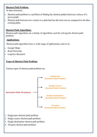
It is important to note the following points regarding Dijkstra Algorithm-
 Dijkstra algorithm works only for connected graphs.
 Dijkstra algorithm works only for those graphs that do not contain any negative weight
edge.
 The actual Dijkstra algorithm does not output the shortest paths.
 It only provides the value or cost of the shortest paths.
 By making minor modifications in the actual algorithm, the shortest paths can be easily
obtained.
 Dijkstra algorithm works for directed as well as undirected graphs.
Dijkstra Algorithm-
dist[S] ← 0 // The distance to source vertex is set to 0
Π[S] ← NIL // The predecessor of source vertex is set as NIL
for all v ∈ V - {S} // For all other vertices
do dist[v] ← ∞ // All other distances are set to ∞
Π[v] ← NIL // The predecessor of all other vertices is set as NIL
S ← ∅ // The set of vertices that have been visited 'S' is initially empty
Q ← V // The queue 'Q' initially contains all the vertices
while Q ≠ ∅ // While loop executes till the queue is not empty
do u ← mindistance (Q, dist) // A vertex from Q with the least distance is selected
S ← S ∪ {u} // Vertex 'u' is added to 'S' list of vertices that have been visited
for all v ∈ neighbors[u] // For all the neighboring vertices of vertex 'u'
do if dist[v] > dist[u] + w(u,v) // if any new shortest path is discovered
then dist[v] ← dist[u] + w(u,v) // The new value of the shortest path is selected
return dist
Implementation-
The implementation of above Dijkstra Algorithm is explained in the following steps-
Step-01:
In the first step two sets are defined-
 One set contains all those vertices which have been included in the shortest path tree.
 In the beginning, this set is empty.
 Other set contains all those vertices which are still left to be included in the shortest path
tree.
 In the beginning, this set contains all the vertices of the given graph.

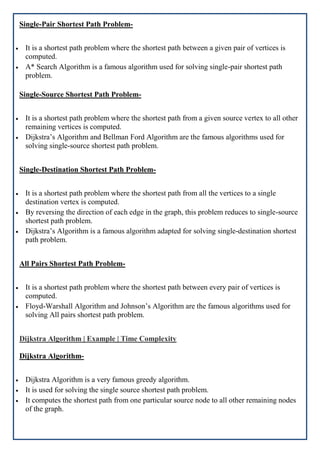
5. Step-02:
For each vertex of the given graph, two variables are defined as-
 Π[v] which denotes the predecessor of vertex ‘v’
 d[v] which denotes the shortest path estimate of vertex ‘v’ from the source vertex.
Initially, the value of these variables is set as-
 The value of variable ‘Π’ for each vertex is set to NIL i.e. Π[v] = NIL
 The value of variable ‘d’ for source vertex is set to 0 i.e. d[S] = 0
 The value of variable ‘d’ for remaining vertices is set to ∞ i.e. d[v] = ∞
Step-03:
The following procedure is repeated until all the vertices of the graph are processed-
 Among unprocessed vertices, a vertex with minimum value of variable‘d’ is chosen.
 Its outgoing edges are relaxed.
 After relaxing the edges for that vertex, the sets created in step-01 are updated.
What is Edge Relaxation?
Consider the edge (a,b) in the following graph-
Here, d[a] and d[b] denotes the shortest path estimate for vertices a and b respectively from
the source vertex ‘S’.
Now,
If d[a] + w < d[b]
then d[b] = d[a] + w and Π[b] = a
This is called as edge relaxation.

6. PRACTICE PROBLEM BASED ON DIJKSTRA ALGORITHM-
Problem-
Using Dijkstra’s Algorithm, find the shortest distance from source vertex ‘S’ to remaining
vertices in the following graph-
Also, write the order in which the vertices are visited.
Solution-
Step-01:
The following two sets are created-
 Unvisited set : {S , a , b , c , d , e}
 Visited set : { }
Step-02:
The two variables Π and d are created for each vertex and initialized as-
 Π[S] = Π[a] = Π[b] = Π[c] = Π[d] = Π[e] = NIL
 d[S] = 0
 d[a] = d[b] = d[c] = d[d] = d[e] = ∞
Step-03:
 Vertex ‘S’ is chosen.
 This is because shortest path estimate for vertex ‘S’ is least.
 The outgoing edges of vertex ‘S’ are relaxed.
Before Edge Relaxation-

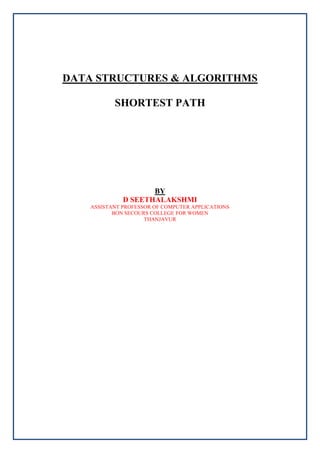
7. Now,
 d[S] + 1 = 0 + 1 = 1 < ∞
∴ d[a] = 1 and Π[a] = S
 d[S] + 5 = 0 + 5 = 5 < ∞
∴ d[b] = 5 and Π[b] = S
After edge relaxation, our shortest path tree is-
Now, the sets are updated as-
 Unvisited set : {a , b , c , d , e}
 Visited set : {S}
Step-04:
 Vertex ‘a’ is chosen.
 This is because shortest path estimate for vertex ‘a’ is least.
 The outgoing edges of vertex ‘a’ are relaxed.

8. Before Edge Relaxation-
Now,
 d[a] + 2 = 1 + 2 = 3 < ∞
∴ d[c] = 3 and Π[c] = a
 d[a] + 1 = 1 + 1 = 2 < ∞
∴ d[d] = 2 and Π[d] = a
 d[b] + 2 = 1 + 2 = 3 < 5
∴ d[b] = 3 and Π[b] = a
After edge relaxation, our shortest path tree is-
Now, the sets are updated as-

9.  Unvisited set : {b , c , d , e}
 Visited set : {S , a}
Step-05:
 Vertex ‘d’ is chosen.
 This is because shortest path estimate for vertex ‘d’ is least.
 The outgoing edges of vertex ‘d’ are relaxed.
Before Edge Relaxation-
Now,
 d[d] + 2 = 2 + 2 = 4 < ∞
∴ d[e] = 4 and Π[e] = d
After edge relaxation, our shortest path tree is-
Now, the sets are updated as-

10.  Unvisited set : {b , c , e}
 Visited set : {S , a , d}
Step-06:
 Vertex ‘b’ is chosen.
 This is because shortest path estimate for vertex ‘b’ is least.
 Vertex ‘c’ may also be chosen since for both the vertices, shortest path estimate is least.
 The outgoing edges of vertex ‘b’ are relaxed.
Before Edge Relaxation-
Now,
d[b] + 2 = 3 + 2 = 5 > 2
∴ No change
After edge relaxation, our shortest path tree remains the same as in Step-05.
Now, the sets are updated as-
 Unvisited set : {c , e}
 Visited set : {S , a , d , b}
Step-07:
 Vertex ‘c’ is chosen.
 This is because shortest path estimate for vertex ‘c’ is least.
 The outgoing edges of vertex ‘c’ are relaxed.
Before Edge Relaxation-

11. Now,
 d[c] + 1 = 3 + 1 = 4 = 4
∴ No change
After edge relaxation, our shortest path tree remains the same as in Step-05.
Now, the sets are updated as-
 Unvisited set : {e}
 Visited set : {S , a , d , b , c}
Step-08:
 Vertex ‘e’ is chosen.
 This is because shortest path estimate for vertex ‘e’ is least.
 The outgoing edges of vertex ‘e’ are relaxed.
 There are no outgoing edges for vertex ‘e’.
 So, our shortest path tree remains the same as in Step-05.
Now, the sets are updated as-
 Unvisited set : { }
 Visited set : {S , a , d , b , c , e}
Now,
 All vertices of the graph are processed.
 Our final shortest path tree is as shown below.
 It represents the shortest path from source vertex ‘S’ to all other remaining vertices.
The order in which all the vertices are processed is :
S , a , d , b , c , e.