Downloaded 395 times
![Introduction to Geophysics Ali Oncel [email_address] Department of Earth Sciences KFUPM Seismic Exploration: Fundamentals 2](https://image.slidesharecdn.com/lecture3-2-091220221439-phpapp01/85/ONCEL-AKADEMI-INTRODUCTION-TO-GEOPHYSICS-1-320.jpg)
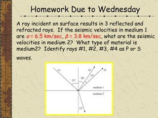
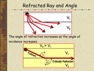
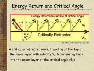
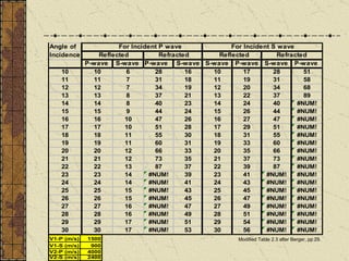
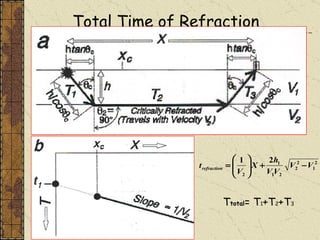
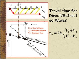
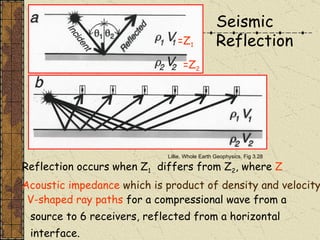
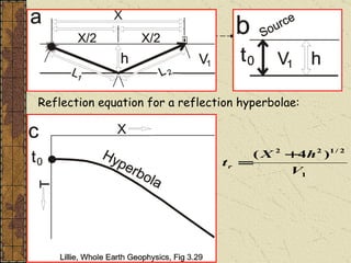
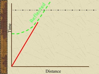
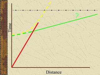
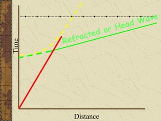
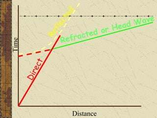
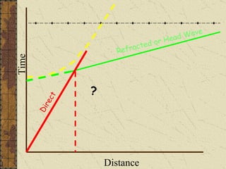
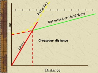
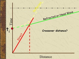

This document provides an introduction to seismic exploration and refraction, including: 1) A ray incident on a surface with two layers results in three reflected and refracted rays, which can be identified as P or S waves based on the velocities in each layer. 2) As the angle of incidence increases, the angle of refraction also increases. 3) At the critical angle, a critically refracted wave travels along the top of the lower layer and leaks energy back into the upper layer. 4) Seismic reflection occurs when the acoustic impedance differs between two layers, producing V-shaped ray paths on a reflection profile.


