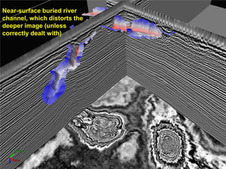
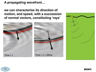
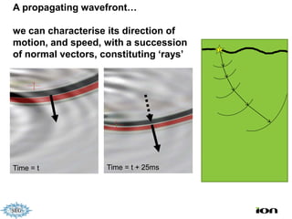
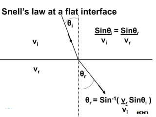
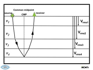
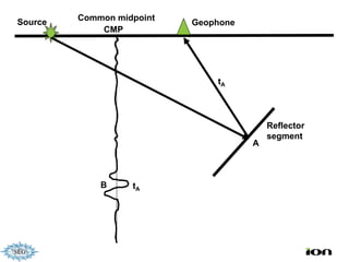
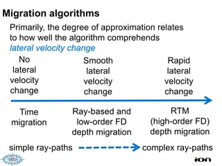
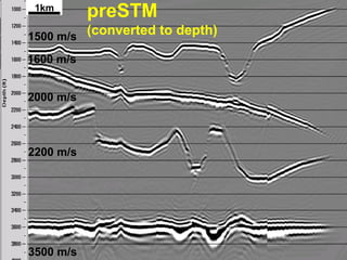
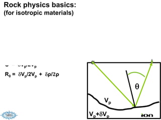
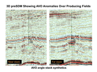
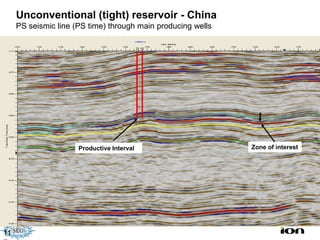
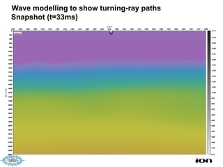
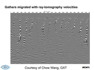
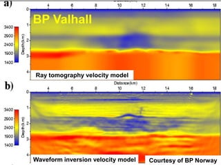
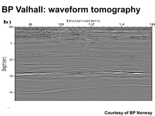
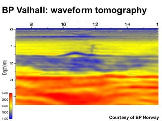
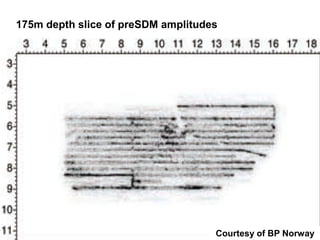
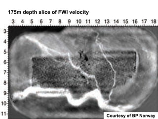
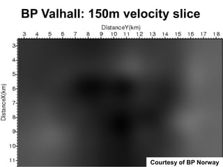
The document discusses the process of hydrocarbon exploration, detailing stages such as data pre-conditioning, velocity model building, migration, and amplitude analysis to locate oil and gas. It explores theoretical concepts, methods, and migration algorithms used in subsurface imaging and presents challenges encountered in seismic data interpretation. The talk emphasizes advancements in strategies like full waveform inversion to enhance accuracy in geological imaging.

1. From Imaging to Inversion
Ian F. Jones
SEG 2012 Honorary Lecture

2. Acknowledgements
 Society of Exploration Geophysicists
 Shell Sponsorship
 ION GX Technology

3. SEG Membership
 SEG Digital Library - full text articles
 Technical Journals in Print and Online
 Networking Opportunities
 Receive Membership Discounts on:
 Continuing Education Courses
 Publications (35% off list price)
 Workshops and Meetings
SEG materials are available today!
Join Online    http://seg.org/join

4. Student Opportunities
 Student Chapters available
 Student Chapter Book Program
 SEG/Chevron Student Leadership Symposium
 Challenge Bowl
 Student Membership Resources
 Scholarships
 SEG/ExxonMobil Student
Education Program
 Annual Meeting Travel Grants
 Student Expos
 the Anomaly newsletter
More information please visit:
   http://seg.org/students

5. From Imaging to Inversion
Ian F. Jones
SEG 2012 Honorary Lecture

6. But before I start…

7. But before I start…
A big thanks to Judy Wall at the
SEG for her sterling work
organizing my schedule !

8. Talk Outline
To a large extent, this presentation is
speculative, in that I’m looking at what ‘might
come next’ moving beyond the current industrial
practise of:
- data pre-conditioning (multiple suppression),
- velocity model building,
- migrating data and then
- analysing amplitude information….

9. Talk Outline
• Hydrocarbon exploration
• Subsurface Imaging
• Waves versus rays
• Velocity model building
• Migration
• Attribute estimation
• Full waveform inversion

10. What is it
that hydrocarbon exploration
geoscientists set out to do …

11. Find oil and gas !

12. But how ?

13. Drill here ???

14. … or here ???

15. How do we decide where to drill?

16. How do we decide where to drill?
… we use sound waves reflecting of the rock
layers to make pictures (similar to ultrasound
medical imaging) and then analyse the amplitude
behaviour of the data to infer what types of rocks
and fluids are present

17. The process currently involves several key
stages:
1) Removal of noise and undesired signal
2) Velocity model building
3) Migration
4) Attribute estimation

18. The process currently involves several key
stages:
1) Removal of noise and undesired signal
2) Velocity model building
3) Migration
4) Attribute estimation

19. Attribute estimation
Once we have estimated the speed of sound
(velocity) in the different rock layers, and then
formed an image from the recorded data
(‘migration’), we can analyse the amplitudes of
the reflections to estimate rock properties
(which helps us distinguish between oil, gas,
water, etc)

20. The geophysical problem
We need to relocate recorded
V1(x,y,z) energy to its ‘true’ position using
an appropriate approximate
solution to the visco-elastic
V2(x,y,z) two-way wave equation
etc
target location
(and what is ‘appropriate’, depends on our objectives)

21. What do these images of
the subsurface look like?

22. Southern North Sea example
Image dimensions are typically several hundred square
kilometres in area, extending to several kilometres depth
Migrated image Sea bed
30km chalk
30km
1600m/s
1800m/s
2000m/s
3000m/s
3500m/s
3.5 km
anhydrite
Gas-bearing layers salt Sound speed in the rocks

23. Near-surface buried river
channel, which distorts the
deeper image (unless
correctly dealt with)

24. How do we describe the way in which
sound travels through the earth?

25. Waves versus Rays

26. Waves versus Rays
The theoretical description of wave phenomena
falls into two categories:
Ray-based
and
Wave- (diffraction or scattering) based
- Both migration and model update depend on
one or other of these paradigms

27. A propagating wavefront…
we can characterise its direction of
motion, and speed, with a succession
of normal vectors, constituting ‘rays’
Time = t Time = t + 25ms

28. A propagating wavefront…
we can characterise its direction of
motion, and speed, with a succession
of normal vectors, constituting ‘rays’
Time = t Time = t + 25ms

29. A propagating wavefront…
we can characterise its direction of
motion, and speed, with a succession
of normal vectors, constituting ‘rays’
Time = t Time = t + 25ms

30. A propagating wavefront…
we can characterise its direction of
motion, and speed, with a succession
of normal vectors, constituting ‘rays’
Time = t Time = t + 25ms

31. A propagating wavefront…
we can characterise its direction of
motion, and speed, with a succession
of normal vectors, constituting ‘rays’
Time = t Time = t + 25ms

32. A propagating wavefront…
we can characterise its direction of
motion, and speed, with a succession
of normal vectors, constituting ‘rays’
Time = t Time = t + 25ms

33. Snell’s law at a flat interface
θi
Sinθi = Sinθr
vi vi vr
vr
θr
θr = Sin-1( vr Sinθi )
vi

34. The high frequency approximation
Seismic wavelength much
smaller than the anomaly
we are trying to resolve
Velocity anomaly
The propagating wavefront can
adequately be described by ray-paths
Snell’s law adequately describes the wave propagation
… ray-based methods (Kirchhoff, beam, …) are OK

35. The high frequency approximation
Seismic wavelength larger or
similar to the anomaly we are
trying to resolve
Small scale-length
velocity anomaly The velocity feature behaves
more like a scatterer than a
simple refracting surface element
Trying to describe the propagation behaviour as
‘rays’ obeying Snell’s law, is no longer appropriate
Ray-based methods (Kirchhoff, beam, …) using the ‘high
frequency approximation’ begin to fail

36. A propagating wavefront…
Time = t Time = t + 25ms Time = t + 50ms
The elements of some velocity features behave more like
point scatterers producing secondary wavefronts

37. Velocity Model Building

38. Common midpoint
source receiver
CMP
v1 Vrms1
v2 Vrms2
v3 Vrms3
v4 Vrms4

39. CMP
Common midpoint gather
CMP
t1 t2 t3 t4 t5
For a CMP gather, we have many
arrival time measurements for a
given subsurface reflector
element

40. CMP
Common midpoint gather
CMP
t1 t2 t3 t4 t5
For a CMP gather, we have many
arrival time measurements for a
given subsurface reflector
element
This curvature is related to the velocity

41.  To estimate velocity for flat layers….

42. Conventional velocity analysis…..
0 Km 5
3.8
S
4.7
Input CMP data

43. Conventional velocity analysis…..
0 Km 5
3.8
Σ
S
4.7
Input CMP data

44. Conventional velocity analysis…..
0 Km 5 Km 5 1.5 2.5 3.5
Km/s
3.8
S
4.7
Input CMP data scan along pick corresponding
trajectories velocity

45.  To estimate velocity for dipping layers….

46.  To estimate velocity for dipping layers….
The notion of the CMP no longer has any meaning,
as the mid-points do not sit above the same
subsurface location for all offsets

47. Dipping layers
Common midpoint
source receiver
CMP
v1 Vrms1
Vrms2
v2
Vrms3
v3 Vrms4

48.  To estimate velocity for dipping layers….
The notion of the CMP no longer has any meaning,
as the mid-points do not sit above the same
subsurface location for all offsets
We have to assess the travel times
for each offset separately

49. Tomographic velocity update…..
Trace raypaths through the current version of
the model and note arrival times

50. Tomographic velocity update…..
Picks of reflection event arrival times synthesized
arrival times from the from ray tracing through
real data the current velocity
model

51. Tomographic velocity update…..
Tomography iteratively modifies the
velocity model so as to minimize the
difference between observed arrival
times on the real data, and ray-traced
times through the current velocity
model

52. Iterative update
(1) PreSDM (2) Autopicker
smooth initial model output migrated gathers Using continuous CRPs, calculate
semblance, velocity & anisotropy
(6) Interpretation (if required) error grids, & RMO stack
Pick constraint layer, insert ‘flood’
velocity, and migrate
(3) TTI Tomography
compute dip field
demigrate picks & RMO stack
update TTI velocity field
remigrate picks & RMO stack
(5) PreSDM
with updated velocity
No
(4) Inversion QC
(4) RMO & z Residual velocity error minimised?
Yes (gathers flat) Depth error acceptable?
acceptable?
Final Volume

53. Iterative update
(1) PreSDM (2) Autopicker
smooth initial model output migrated gathers Using continuous CRPs, calculate
semblance, velocity & anisotropy
(6) Interpretation (if required) error grids, & RMO stack
Pick constraint layer, insert ‘flood’
velocity, and migrate
This process (3) TTI Tomography
usually involves demigrate picksdipRMO stack
compute
&
field
6-8 iterations update TTI velocity field
remigrate picks & RMO stack
(5) PreSDM
with updated velocity
No
(4) Inversion QC
(4) RMO & z Residual velocity error minimised?
Yes (gathers flat) Depth error acceptable?
acceptable?
Final Volume

54. Iteration 1, 3D preSDM
0
Top Chalk
k
m
2

55. Iteration 2, 3D preSDM
0
Top Chalk
k
m
2

56. Iteration 3, 3D preSDM
0
Top Chalk
k
m
2

57. Iteration 1 Velocities
0
k
m
2

58. Iteration 2 Velocities
0
k
m
2

59. Iteration 3 Velocities
0
k
m
2

60. Migration:
putting the recorded data
back where it came from

61. Common midpoint
source receiver
CMP
v1 Vrms1
v2 Vrms2
v3 Vrms3
v4 Vrms4

62. Common midpoint
source receiver
CMP
v1 Vrms1
v2 Vrms2
v3 Vrms3
v4 Vrms4

63. Plot all the traces from various common midpoints to
form a picture of the subsurface…

64. Common midpoint
Source Geophone
CMP
tA
Reflector
segment
A
B tA

65. Common midpoint
Source Geophone
CMP
tA
Reflector
segment
A
B tA
‘Migration’ moves the recorded data
back to where it came from

66. Main migration algorithms in use today
- Kirchhoff
Ray - Beam
- (GB, CRAM, CRS, CFP, ….)
- Wavefield extrapolation (WEM)
Wave
- Reverse-Time (two-way)

67. Migration algorithms
relocate recorded energy to its ‘true’ position
using an appropriate approximate solution to the
two-way visco-elastic wave equation (but what is
‘appropriate’, depends on our objectives)

68. Migration algorithms
Primarily, the degree of approximation relates
to how well the algorithm comprehends
lateral velocity change

69. Migration algorithms
Primarily, the degree of approximation relates
to how well the algorithm comprehends
lateral velocity change
No Smooth Rapid
lateral lateral lateral
velocity velocity velocity
change change change

70. Migration algorithms
Primarily, the degree of approximation relates
to how well the algorithm comprehends
lateral velocity change
No Smooth Rapid
lateral lateral lateral
velocity velocity velocity
change change change
Time Ray-based and RTM
migration low-order FD (high-order FD)
depth migration depth migration

71. Migration algorithms
Primarily, the degree of approximation relates
to how well the algorithm comprehends
lateral velocity change
No Smooth Rapid
lateral lateral lateral
velocity velocity velocity
change change change
Time Ray-based and RTM
migration low-order FD (high-order FD)
depth migration depth migration
simple ray-paths complex ray-paths

72. 1km
Velocity-depth model
1490 m/s
1600 m/s
2000 m/s
2200 m/s
3500 m/s

73. Acoustic shot gather 3km 6km
1s
Energy travelling in the
water (the ‘direct’ wave)
Reflection from
water bottom
3s
Reflections from 4s
deeper rock layers
5s

74. 1km
Velocity-depth model
1490 m/s
1600 m/s
2000 m/s
2200 m/s
3500 m/s

75. 1km
preSDM
1500 m/s
1600 m/s
2000 m/s
2200 m/s
3500 m/s

76. 1km
preSTM
1500 m/s (converted to depth)
1600 m/s
2000 m/s
2200 m/s
3500 m/s

77. Migration Issues:
Lateral velocity variation:
Kirchhoff preSTM
vs Kirchhoff preSDM
vs RTM
Norwegian Sea shallow water gas example

78. Interval velocity model
Autopicking @50*50m 1km Courtesy of ConocoPhillips Norway
Tomo @250*250*50m

79. Kirchhoff preSTM (initial model)
1km Courtesy of ConocoPhillips Norway

80. Kirchhoff preSDM
Autopicking @50*50m 1km Courtesy of ConocoPhillips Norway
Tomo @250*250*50m

81. RTM
Autopicking @50*50m 1km Courtesy of ConocoPhillips Norway
Tomo @250*250*50m

82. Migration Issues:
In addition to the degree of
lateral velocity change, we also
have the issue of ray-path
complexity to consider in the
migration…

83. Migration Issues:
Multi-pathing:

84. What is multi-pathing?
There is more than one path from a surface location to a
subsurface point
salt
A Kirchhoff scheme usually only computes travel times for
one ray path… what happens to the energy from the rest
of the ray paths from input data?

85. Migration Issues:
Multi-pathing:
Kirchhoff vs WEM
North Sea shallow water diapir example

86. 1km
salt
2
km
4
6
Vi(z)

87. 1km
2
km
4
6
Anisotropic Kirchhoff 3D preSDM

88. 1km
2
km
4
6
Anisotropic one-way SSFPI (WEM) 3D preSDM

89. Migration Issues:
Two-way propagation:

90. What is two-way propagation?
Conventional one-way propagation Two-way propagation: requires a more
as assumed by standard migration complete solution of the wave equation
schemes to migrate such arrivals
Nor from the
reflection point
back up to the
surface The direction of propagation changes
either on the way down from the surface
No change in propagation
to the reflection point, or from the
direction on the way from
reflection point back up to the surface
the surface down to the
reflection point

91. Migration Issues:
Two way ray paths:
WEM vs RTM
North Sea shallow water diapir example

92. 1km
2
km
4
6
Anisotropic one-way SSFPI (WEM) 3D preSDM

93. 1km
2
km
4
6
Anisotropic two-way RTM 3D preSDM

94. 1km
2
km
4
6
Anisotropic two-way RTM 3D preSDM

95. Migration Issues:
Two way ray paths:
WEM vs RTM
West African deep water diapir example

96. WEM
1km
1km

97. RTM
1km
1km

98. RTM
1km
1km

99. RTM
1km
1km

100. RTM
1km
1km

101. Once we have estimated velocity, and
migrated the data to obtain gathers in
their correct spatial location, we can
begin to analyse amplitude
information

102. Extracting other rock attributes
(as well as velocity):
rock type, fluid type, density,
saturation, pressure, attenuation, ….

103. Rock physics basics:
(for isotropic materials)
Stress (pressure) = force/area = F/A
Strain = fractional change in volume = dV/V
Bulk modulus = pressure/strain = B = - (F/A)/(dV/V)
Compressibility = 1/B
B = λ + 2/3 μ

104. Common midpoint gather
CMP
t1 t2 t3 t4 t5
For a CMP gather, we have many
arrival time measurements for a
given subsurface reflector
element

105. Common image gather
CIG or CRP
t1 t2 t3 t4 t5 offset
After depth migration with an
acceptable velocity model, all
events in the gather should
line-up  ‘flat gathers’
Migrated depth

106. Having obtained estimates of velocity:
we can then estimate other parameters from
amplitude behaviour

107. Gathers output from preSDM - not exactly flat

108. After final residual event alignment and noise suppression
These data are
now suitable for
analyzing
variations in
amplitude:

109. After final residual event alignment and noise suppression
These data are
now suitable for
analyzing
variations in
amplitude:
vertically from
reflector-to-
reflector:
(ρ2v2 – ρ1v1)/(ρ2v2 + ρ1v1)

110. After final residual event alignment and noise suppression
These data are
now suitable for
analyzing
variations in
amplitude:
vertically from
reflector-to-
reflector
and laterally
versus incidence
angle at the
reflectors

111. Incident P wave
Transmitted P wave
Reflected P wave
text
The Knott-Zoeppritz equations relate the
amplitude change as a function of incident
angle, to Vp, Vs, and density

112. Rock physics basics:
(for isotropic materials)
θ
Vp
Vp+δVp

113. 3D preSDM Showing AVO Anomalies Over Producing Fields
Near stack Far stack
AVO angle stack synthetics

114. 3D preSDM Showing AVO Anomalies Over Producing Fields
Near stack (0º-25º) Far stack (25º-50º)
Average absolute amplitude Top Balder +50 - +200

115. MacCulloch
15/24b-6 Far-angle stack EI Inversion
N S W E
15/24b-6
15/24b-6
Top
Balder
Low EI Oil 650
Sand 600
550
500
450

116. N 15/25b-3 S
Top Balder
Brenda
Field
650
600
Possible low EI Oil Sand on flank? 550
500
15/25b-3 Far-stack Inversion (inline) 450

117. Unconventional (tight) reservoir - China
PS seismic line (PS time) through main producing wells
Productive Interval Zone of interest
11

118. Unconventional (tight) reservoir - China
Characterizing Lithological Variations
shale sand
Record P-wave only
Impute shear-wave measurement
using simultaneous inversion (AVO)
Attempt to infer sand-shale variations
Record shear-waves directly
More accurate depiction of
sand-shale variations
11

119. Unconventional (tight) reservoir - China
Full-wave explains well productivity – fracture characterization
Same lithology Note presence of
No fractures fractures in
No production producing zone
New well location
11

120. What we’ve reviewed so far, has
been the ‘state of the art’:
1) velocity model building
2) migration
3) attribute estimation

121. What next?
Can we do all this in one step?
= full elastic waveform inversion

122. To accomplish this task, we must accurately
model the behaviour of the recorded data:

123. To accomplish this task, we must accurately
model the behaviour of the recorded data:
- we start with initial estimates of the rock physics
parameters (P-wave velocity, S-wave velocity,
density, anisotropy, absorption, ..)

124. To accomplish this task, we must accurately
model the behaviour of the recorded data:
- we start with initial estimates of the rock physics
parameters (P-wave velocity, S-wave velocity,
density, anisotropy, absorption, ..)
- make synthetic data and compare it to the real
data

125. To accomplish this task, we must accurately
model the behaviour of the recorded data:
- we start with initial estimates of the rock physics
parameters (P-wave velocity, S-wave velocity,
density, anisotropy, absorption, ...)
- make synthetic data and compare it to the real
data
- iteratively adjust the parameters until modelled
and real data match

126. Real shot Modelled shot
- = residual

127. Recall the conventional approach:
(Tomographic velocity update)…..
Tomography iteratively modifies the
velocity model so as to
minimize the difference
between observed arrival times on the real
data, and ray-traced times through the
current velocity model

128. Waveform inversion update…..
Waveform inversion iteratively modifies
the parameter model so as to
minimize the difference
between observed amplitudes on the real
data, and modelled amplitudes created
using the current parameter model

129. What’s involved in getting the amplitude right?
-Visco elastic wave propagation (incorporates
attenuation and shear modes)
-Elastic wave propagation (shear modes)
-Acoustic wave propagation (P-wave only, thus
ignoring density)
-Anisotropy
-Source wavelet (and are ghosts present?)
-Source wavelet time delay
-Cycle skipping (offset and frequency dependent)

130. Ignoring density
Reflection strength (amplitude) is related to impedance
contrast:
(ρ2v2 – ρ1v1)/(ρ2v2 + ρ1v1)
By ignoring density, we are saying that impedance is
only a function of P velocity:
Thus, if we invert using reflection events, we will have
an amplitude error
So, to avoid this error perhaps use only refractions
(diving, turning waves)

131. Where are the refractions?
Perform some forward modelling to assess how deeply
the diving waves penetrate
The region of validity of the model update will be
related to this depth of penetration

132. Raytracing to show turning-ray paths
- expected maximum depth of WFI update
10km cable
H2O
Observed depth of
update Insert Velocity Model Here with Rays for Cable we are using
Maximum expected depth
of WFI update
Ray tracing performed in tomography
derived sediment flood model

133. Wave modelling to show turning-ray paths
Snapshot (t=33ms)

134. Wave modelling to show turning-ray paths
Snapshot (t=1407ms)

135. Wave modelling to show turning-ray paths
Snapshot (t=1865ms)

136. Wave modelling to show turning-ray paths
Snapshot (t=2454ms)

137. Wave modelling to show turning-ray paths
Snapshot (t=3272ms)
Max Depth of Turning Rays ~3400m
for cable length

138. Do we obtain a better earth-model parameters?
One way to confirm if FWI has produced better earth-
model parameters is to use the FWI velocity to perform
a new migration

139. Gathers migrated with ray-tomography velocities
Courtesy of Chow Wang, GXT

140. Gathers migrated with waveform inversion velocities
Courtesy of Chow Wang, GXT

141. Shallow Section Before WFI
Courtesy of Chow Wang, GXT

142. Shallow Section After WFI
Courtesy of Chow Wang, GXT

143. BP in-house project: Valhall
(courtesy of Jan Kommedal & Laurent Sirgue)
Courtesy of BP Norway

144. BP Valhall
Ray tomography velocity model
Waveform inversion velocity model Courtesy of BP Norway

145. BP Valhall: ray-based tomography
Courtesy of BP Norway

146. BP Valhall: waveform tomography
Courtesy of BP Norway

147. BP Valhall: waveform tomography
Courtesy of BP Norway

148. 175m depth slice of preSDM amplitudes
Courtesy of BP Norway

149. 175m depth slice of FWI velocity
Courtesy of BP Norway

150. BP Valhall: 150m velocity slice
Courtesy of BP Norway

151. BP Valhall: 150m velocity slice
Courtesy of BP Norway

152. BP Valhall: 1050m velocity slice
Courtesy of BP Norway

153. BP Valhall: 1050m velocity slice
Courtesy of BP Norway

154. The ultimate goal of full waveform inversion….
At present, the limiting assumptions we make
in waveform inversion limit what we can
achieve:
we can currently forward model with a priori
parameters for: density, attenuation, anisotropy
(and perhaps Vs) but
invert only for P-wave velocity

155. The ultimate goal of full waveform inversion….
IFF we can move beyond the present limiting
assumptions, then we may be able to invert so
as to update all these parameters thereby
recovering density, Vp, Vs, Q, and other
parameters.
Interpretation would then be performed on
these parameter fields directly, rather than on
inversions of migrated data obtained using the
velocity parameter

156. The ultimate goal of full waveform inversion….
Vp Vs ρ ε δ
model
Inversion
result
Courtesy of Olga Podgornova

157. The ultimate goal of full waveform inversion….
Courtesy of Joachim Mispel & Ina Wenske

158. The ultimate goal of full waveform inversion….
Vp
Vs/10
Vs
Courtesy of Satish Singh

159. In other words ….

160. Move from this
lengthy disjointed
process……

161. Extensive data pre-processing (remove multiples)
Move from this
lengthy disjointed
process……

162. Extensive data pre-processing (remove multiples)
Move from this
lengthy disjointed
process……
+ Iterative velocity model update and migration

163. Extensive data pre-processing (remove multiples)
Move from this
lengthy disjointed
process……
+ Iterative velocity model update and migration
+ elastic
parameter
inversion

164. Extensive data pre-processing (remove multiples)
Move from this
lengthy disjointed
process……
+ Iterative velocity model update and migration
+ elastic
parameter
inversion
+ rock
property
estimation

165. To this ……

166. CLEAN INPUT DATA
(including multiples)
To this ……
FWI
rock
properties

167. But perhaps we shouldn’t
‘hold our breath’
just yet !

168. Thank you !