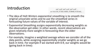
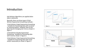
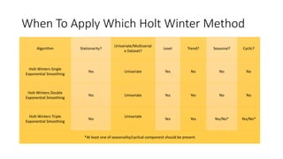
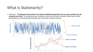
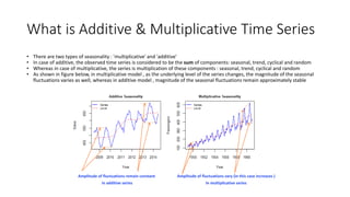
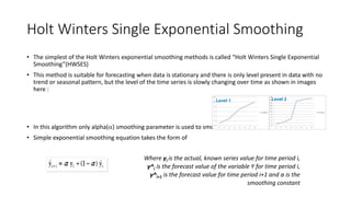
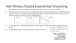
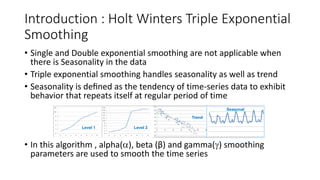
The document provides an overview of Holt-Winters exponential smoothing methods for time series forecasting, categorizing them into three types: single, double, and triple exponential smoothing, each suitable for different data patterns like trend and seasonality. It explains key concepts such as stationarity, level, and the distinction between additive and multiplicative time series components. Furthermore, it highlights the importance of selecting appropriate smoothing parameters to improve forecast accuracy, using examples to demonstrate the application of each method.

1. TIME SERIES FORECASTING
HOLT WINTERS EXPONENTIAL SMOOTHING
A Simplistic Explainer Series For Citizen Data Scientists
J o u r n e y T o w a r d s A u g m e n t e d A n a l y t i c s

2. Introduction &
Terminologies

3. Introduction
• The idea of Holt Winters exponential smoothing is to smooth the
original univariate series and to use the smoothed series in
forecasting future values of the variable of interest.
• Exponential Smoothing assigns exponentially decreasing weights as
the observation get older. In other words, recent observations are
given relatively more weight in forecasting than the older
observations.
• For example, Imagine a weighted average where we consider all of the
data points, while assigning exponentially smaller weights as we go
back in time. For example if we started with 0.9, our weights would be
(going back in time):

4. Introduction
Holt Winters Algorithms are applied when
data is stationary.
Basically, there are three types of Holt
Winters Exponential Smoothing methods :
1.Holt Winters Single Exponential Smoothing
: Suitable for forecasting data with no trend
or seasonal pattern. However level of the
data may be changing over time as shown in
figure 1
2.Holt Winters Double Exponential
Smoothing : Suitable for forecasting data
with trend as shown in figure 2.
3.Holt Winters Triple Exponential Smoothing
: Suitable for forecasting data with trend
and/or seasonality as shown in figure 2. TREND
SEASONAL
LEVEL
Level 1
Level 2
Level 3
Figure 1
Figure 2

5. When To Apply Which Holt Winter Method
Algorithm Stationarity?
Univariate/Multivariat
e Dataset?
Level Trend? Seasonal? Cyclic?
Holt-Winters Single
Exponential Smoothing
Yes Univariate Yes No No No
Holt-Winters Double
Exponential Smoothing
Yes Univariate Yes Yes No No
Holt-Winters Triple
Exponential Smoothing
Yes
Univariate
Yes Yes Yes/No* Yes/No*
*At least one of seasonality/cyclical component should be present

6. What Is Stationarity?
• Definition : “A stationary time series is one whose statistical properties such as mean, variance are all
constant over time.” In a practical sense, stationary series vary around a constant mean level, neither
decreasing nor increasing systematically over time, with constant variance.
Stationaryseries
Nonstationaryseries
Mean is constant
Variance is constant
Mean is not constant
Variance is not constant

7. What Is Level?
Level : In a time series there might be one or more significant jump, occurring in few successive time points. Post the jump the level of a time
series is different compared to the one before jump. If there is no significant jump, we say the time series has level 1, else more than one
depending on the number of considerable jump(s) as explained in the diagrams below
Level 1
Level 2
Level 3

8. What is Additive & Multiplicative Time Series
• There are two types of seasonality : 'multiplicative' and 'additive'
• In case of additive, the observed time series is considered to be the sum of components: seasonal, trend, cyclical and random
• Whereas in case of multiplicative, the series is multiplication of these components : seasonal, trend, cyclical and random
• As shown in figure below, in multiplicative model , as the underlying level of the series changes, the magnitude of the seasonal
fluctuations varies as well, whereas in additive model , magnitude of the seasonal fluctuations remain approximately stable
Amplitude of fluctuations remain constant
in additive series
Amplitude of fluctuations vary (in this case increases )
In multiplicative series

9. Holt-Winters Single Exponential Smoothing

10. Introduction with
Example

11. Holt Winters Single Exponential Smoothing
• The simplest of the Holt Winters exponential smoothing methods is called “Holt Winters Single Exponential
Smoothing”(HWSES)
• This method is suitable for forecasting when data is stationary and there is only level present in data with no
trend or seasonal pattern, but the level of the time series is slowly changing over time as shown in images
here :
• In this algorithm only alpha() smoothing parameter is used to smooth the time series
• Simple exponential smoothing equation takes the form of
Where yi is the actual, known series value for time period i,
y^i is the forecast value of the variable Y for time period i,
y^i+1 is the forecast value for time period i+1 and α is the
smoothing constant
Level 1 Level 2

12. Example-HWSES
• For example, The Bay City Seafood Company recorded the monthly
cod catch for the previous two years, as given below.
• The plot of these data suggests that there is no trend or seasonal
pattern but a single level present in data as shown in graph below :
Monthly Cod Catch
250
270
290
310
330
350
370
390
410
0 5 10 15 20 25
Month
CodCatch(intons)
LEVEL = 1
Actual Cod Catch
Month Cod
M1 362
M2 381
M3 317
M4 297
M5 399
M6 402
M7 375
M8 349
M9 386
Input dataset

13. Example-HWSES
• As there is no trend / seasonality but only level
present in data , we should choose holt winters
single exponential smoothing method for
forecasting
• Find an optimum value of  for which model
gives minimum value for MAPE (Mean absolute
percentage error) in order to get better accuracy
• After the HWSES model is run , it will provide
forecasted values of target variable(code catch
in this case) for user specified periods ahead ,
let’s say 5 as shown in blue box in table:
Actual Cod Catch
Month Cod
M1 362
M2 381
M3 317
M4 297
M5 399
M6 402
M7 375
M8 349
M9 386
Forecasted Cod Catch
M10 380
M11 399
M12 378
M13 352
M14 389
Forecasted values

14. Model Accuracy :
Actual Predicted Abs((Actual - predicted)/actual)*100
M10 399 380 4.76
M11 402 399 0.75
M12 375 378 0.80
M13 349 352 0.86
M14 386 389 0.78
MAPE = Sum(Y1 to Y5) = 7.94
Accuracy = ABS (1-7.94)*100 = 92
MAPE = 8%
Hence accuracy = 100-MAPE = 92% , So model is accurate
Along with forecasted values, MAPE and prediction accuracy is displayed so user knows how much accurate the forecasts
are.
How MAPE and Accuracy is calculated is explained below :
MAPE :
Where yt is the actual, known series value for time period t,
y^t is the forecast value of the variable Y for time period t
N is number of observations
Using this formula , MAPE can be calculated for 5 months ahead forecasts using recent most
5 months data as follows:

15. Standard Tuning
Parameters

16. Standard Tuning Parameters
• Model approach & parameters:
• In Holt Winters, there are two approaches to fitting a model : Automatic and Manual
• Which smoothing parameters are going to be used depends on the data pattern and their values
lie between 0 and 1
• In case of single exponential smoothing, there is a provision to select only alpha. When alpha is
automatically selected by system than it’s called auto fit model and when alpha is manually input
by user than it’s called fit model
• Ideally automatic approach should be chosen as in this approach, model automatically choses and
applies the right algorithm and parameters based on the nature of data
• A high value of alpha will lead to the majority of the weight being placed on the most recent
observations whereas a low value of alpha will mean that observations further in the past will gain
more importance. A value of alpha = 1 will obviously make the forecast equal to the final value of
the series
• Forecast period :
• For both type of approaches , user has to input the forecast period value.
• For example, if user wants to predict the sales value for 10 periods ahead then this value should
be input as 10

17. Sample UI for
input/tuning
parameters and output

18. Sample UI for selecting Inputs and applying tuning
parameters
Select the variables you would
like to Forecast
Date
GDP Value
If user changes the approach to Manual then
this box should be displayed , showing
additional provision to set alpha value
Tuning parameters
Approach
Forecast Period
Automatic
Approach
Forecast
Period
Alpha
Manual
By default this box should be displayed
with default approach as Automatic and
provision to select forecast periods
Select the time stamp
Date
GDP Value

19. Sample UI for output
Output will be forecasted values based on user specified
time period along with line charts showing actual and
forecasted series and prediction accuracy
Timestamp Observed values
M1 125
M2 130
M3 145
M4 150
M5 170
M6 240
Timestamp Forecasted values
M7 170
M8 220
M9 230
M10 235
M11 240

20. Limitations

21. Limitations
• Holt Winters Exponential Smoothing Algorithms are used only when
data series is stationary
• Holt Winters Single Exponential Smoothing is used for forecasting
data with only levels and in real life data this is hardly the case
• Holt winter is only for univariate data forecasts

22. Business Use case

23. Use case
• Business problem :
• Forecasting number of viewers by day for a particular game show for next
two months
• Input data: Last six months daily viewer count data
• Data pattern : Data taken as an input exhibit stationarity and no trend
/seasonality
• Business benefit:
• Helps in planning for repeat telecast
• Can pitch in for more advertisement (fund raise) if projected count of
viewers are high
• Improvement planning can be done for the game show to
increase/maintain the level of popularity

24. Holt-Winters Double
Exponential Smoothing

25. Introduction with
Example

26. Holt Winters Double Exponential Smoothing
1. Simple exponential smoothing is not applicable when there is a trend in the data
2. Double exponential smoothing is a single exponential smoothing applied twice to both level and
trend and hence is suitable for forecasting when data is stationary and there is level and trend
pattern present in data as shown in images below:
3. In this algorithm , alpha() and beta (β) smoothing parameters are used to smooth the time
series
4. Double exponential smoothing equation takes the form of:
Level 1 Level 2 Trend
Where, Lt is level at time t,
 Is weight for the level,
Tt trend at time t,
𝜷 is weight for the trend,
Yt is fitted values at time t

27. Example-HWDES
• Let’s take an example of Thermostat sales recorded weekly as given below :
• The plot of these data suggests that there is an
• overall an upward trend, the growth rate
• has been increasing over the period of 52-weeks and
• there is no seasonal pattern as shown in graph below :
Input dataset
TREND
Actual sales
Week Sales
W1 206
W2 245
W3 185
W4 169
W5 192
W6 177
W7 207
W8 216
W9 193
Forecasted sales
W10 190
W11 180
W12 202
W13 209
W14 204
LEVEL 2LEVEL 1
sales

28. Example-HWDES
• As there is no seasonality but two levels and upward
trend present in data , we should choose holt winters
double exponential smoothing method for forecasting.
• Find an optimum value of  and β for which model
gives minimum value for MAPE (Mean absolute
percentage error) in order to get better accuracy.
• After the HWDES model is run , it will provide
forecasted values of target variable( Thermostat sales
in this case) for user specified periods ahead , let’s say
5 as shown in blue text in table:
Input dataset
Forecasted values
Actual sales
Week Sales
W1 206
W2 245
W3 185
W4 169
W5 192
W6 177
W7 207
W8 216
W9 193
Forecasted sales
W10 190
W11 180
W12 202
W13 209
W14 204

29. Model Accuracy
• Along with forecasted values, MAPE and prediction accuracy is displayed so user knows how much accurate the forecasts
are.
• How MAPE and Accuracy is calculated is explained below :
• Using this formula , MAPE can be calculated for 5 weeks ahead forecasts using recent most 5 weeks data as follows:
MAPE :
Where yt is the actual, known series value for time period t,
y^t is the forecast value of the variable Y for time period t
N is number of observations
MAPE = 14%
Hence accuracy = 100-MAPE = 86% , So model is accurate
#Week Actual Y Predicted Y^ Abs((Actual - predicted)/actual)*100
W10 192 190 1.04
W11 177 180 1.69
W12 207 202 2.42
W13 216 209 3.24
W14 193 204 5.70
MAPE = Sum(W5 to W9) =14
Accuracy =100-MAPE=86

30. Standard Tuning
Parameters

31. Standard tuning parameters
Model approach &
parameters:
In Holt Winters, there are two approaches to fitting a model : Automatic and
Manual.
Which smoothing parameters are going to be used depends on the data
pattern and their values lie between 0 and 1.
In case of double exponential smoothing, there is a provision to select alpha
for level and beta for trend. When alpha & beta is automatically selected by
system than it’s called automatic approach and when alpha & beta is manually
input by user than it’s called manual approach.
Ideally automatic approach should be chosen as in this approach, model
automatically choses and applies the right algorithm and parameters based on
the nature of data.
Forecast period :
For both type of approaches , user has to input the forecast period value.
For example, if user wants to predict the sales value for 10 periods ahead then
this value should be input as 10.

32. Sample UI For
Input/Tuning
Parameters And Output

33. Sample UI for selecting Inputs and applying tuning parameters
Select the variables you would
like to Forecast
Date
Sales
If user changes the approach to Manual then this
box should be displayed , showing additional
provision to set alpha and beta values
Tuning parameters
Approach
Forecast Period
Automatic
Approach
Forecast
Period
Alpha
Beta
Manual
By default this box should be displayed with default approach
as Automatic and provision to select forecast periods
Select the time stamp
Date
Sales

34. Sample UI for output
Output will be forecasted values based on user specified
time period along with line charts showing actual and
forecasted series and prediction accuracy.
Timestamp Observed values
W1 192
W2 200
W3 207
W4 216
W5 193
Timestamp Forecasted values
W6 230
W7 212
W8 192
W9 192
W10 196

35. Limitations

36. Limitations
• Holt Winters Double Exponential Smoothing is used for forecasting
data consisting only level and trends . In case of seasonality this
algorithm is not applicable
• Holt winter double exponential smoothing is only for univariate and
stationary data forecasts

37. Business use case

38. Business use case
• Business problem :
• Insurance claim manager wants to forecast policy sales for next month
based on past 12 months data
• Data pattern : Input data exhibits stationarity , level and strong upward
trend but no seasonality
• Business benefit:
• If projected claims are lower than expected then proper marketing strategy
can be devised to improve sales
• Competition policy can be analyzed in terms of what all perks and benefits
they provide to customers and existing policy can be modified to increase
the market share

39. Holt-Winters Triple Exponential
Smoothing

40. Introduction with
Examples

41. Introduction : Holt Winters Triple Exponential
Smoothing
• Single and Double exponential smoothing are not applicable when
there is Seasonality in the data
• Triple exponential smoothing handles seasonality as well as trend
• Seasonality is defined as the tendency of time-series data to exhibit
behavior that repeats itself at regular period of time
• In this algorithm , alpha(), beta (β) and gamma() smoothing
parameters are used to smooth the time series
Level 1 Level 2
Trend
Seasonal

42. Example : Holt Winters Triple Exponential
Smoothing
• Let’s take an example of year wise sports drink sales observations :
• The plot of these data suggests that there is linear upward trend
over the 5 years period, magnitude of the seasonal span increases
as the level of the time series increases as shown in figure below
• Hence, we can choose holt winters triple multiplicative algorithm
for forecasting
Actual Sales
Years Sales
Y1 70
Y2 150
Y3 190
Y4 210
Y5 250
Y6 290
Y7 310
Y8 390
Y9 400
Y10 420
Forecasted sales
Y11 289
Y12 315
Y13 400
Y14 419
Y15 420

43. Example : Holt Winters
Triple Exponential
Smoothing
Find an optimum value of , β and  for
which model gives minimum value for MAPE
(Mean absolute percentage error) in order to
get better accuracy
After the HWTES model is run , it will provide
forecasted values of target variable(Sports
drink sales in this case) for user specified
periods ahead , let’s say 5 as shown in blue
text in table:
Forecasted values
Actual Sales
Years Sales
Y1 70
Y2 150
Y3 190
Y4 210
Y5 250
Y6 290
Y7 310
Y8 390
Y9 400
Y10 420
Forecasted sales
Y11 289
Y12 315
Y13 400
Y14 419
Y15 420

44. Example : Holt Winters Triple Exponential
Smoothing
• Along with forecasted values, MAPE and prediction accuracy is displayed so user knows how
much accurate the forecasts are
• How MAPE and Accuracy is calculated is explained below :
• Using this formula , MAPE can be calculated for 5 years ahead forecasts using recent most 5 years
data as shown in table below:
MAPE :
Where Yt is the actual, known series value for time period t,
Y^t is the forecast value of the variable Y for time period t
N is number of observations
MAPE = 9%
Hence accuracy = 100-MAPE = 91% , So model is
accurate
Years Actual Y Predicted Y^ Abs((Actual - predicted)/actual)*100
Y11 290 289 0.34
Y12 310 315 1.61
Y13 390 400 2.56
Y14 400 419 4.75
Y15 420 420 0.00
MAPE = Sum(M6 to M10) =09
Accuracy =100-MAPE=91

45. Standard Tuning
Parameters

46. Standard tuning parameters
Model approach &
parameters:
In Holt Winters, there are two approaches to fitting a model :
Automatic and Manual
Which smoothing parameters are going to be used depends on
the data pattern and their values lie between 0 and 1
In case of triple exponential smoothing, there is a provision to
select alpha for level, beta for trend and gamma for seasonal.
When alpha, beta and gamma are automatically selected by
system than it’s called automatic approach and when alpha, beta
and gamma are manually input by user than it’s called manual
approach
Ideally automatic approach should be chosen as in this
approach, model automatically chooses and applies the right
algorithm and parameters based on the nature of data
Method:
Additive/multiplicative should be chosen automatically using
MAPE value. Whichever model has lower MAPE should be
chosen for forecasts
Forecast period :
For both type of approaches , user has to input the forecast
period value
For example, if user wants to predict the sales value for 10
periods ahead then this value should be input as 10

47. Sample UI For
Input/Tuning
Parameters And Output

48. Sample UI for selecting Inputs and applying tuning
parameters
Select the variables you would
like to Forecast
Year
Sports Drink Sales
If user changes the approach to Manual then this
box should be displayed , showing additional
provision to set alpha, beta and gamma values
Tuning parameters
Approach
Forecast
Period
Method
Automatic
Approach
Forecast
Period
Alpha
Beta
Gamma
Manual
By default this box should be displayed
with default approach as Automatic and
provision to select forecast periods
Select the time stamp
Year
Sports Drink Sales
Multiplicative

49. Sample UI for output
Output will be forecasted values based on user
specified time period along with line charts showing
actual and forecasted series and prediction
accuracy.
Timestamp Observed values
Y1 10
Y2 15
Y3 17
Y4 20
Y5 25
Timestamp Forecasted values
Y6 12
Y7 16
Y8 18
Y9 22
Y10 27
Additive
Multiplicative

50. Limitations

51. Limitations
1.Holt Winters triple exponential smoothing can not handle irregular
pattern well.
2.Holt winter triple exponential smoothing is only for univariate and
stationary data forecasts.

52. Business use case

53. Business use case
• Business problem :
• A power generator company wants to predict the electricity demand
for next two months based on past 2 years’ daily power consumption
data
• Data pattern : Input data exhibits stationarity , trend and seasonality
• Business benefit:
• A power generator company can make use of these forecasts for the
control and scheduling of power systems
• It widely helps in balancing supply and demand

54. Want to Learn
More?
Get in touch with us @
support@Smarten.com
And Do Checkout the Learning section
on
Smarten.com
June 2018