SEASONAL
DECOMPOSITION OF TIME
SERIES DATA IN MACHINE
LEARNING
Decomposing Time Series into Trend, Seasonal,
and Residual Components using Real-World Data
For Any Assignment Related Queries Reach Us At:
Email: - support@programminghomeworkhelp.com or
Website: - https://www.programminghomeworkhelp.com/
SEASONAL DECOMPOSITION OF
TIME SERIES DATA
Welcome to the sample assignment from programminghomeworkhelp.com
where we simplify Seasonal decomposition of time series data is a
fundamental technique in time series analysis, used to understand and
interpret the underlying patterns in datasets. This method involves breaking
down a series into three main components: trend, seasonal, and residual.
By doing so, it helps to isolate long-term movements, recurring patterns,
and irregular variations. In this assignment, we will explore these concepts
and apply them to a real-world dataset. For additional support and
resources, Programming Homework Help provides expert guidance and
solutions tailored to various programming and data analysis challenges.
Problem:
Explain the concept of seasonal decomposition of time series data. How
would you decompose a time series into its trend, seasonal, and residual
components? Provide an example using a real-world dataset.
Solution:
Seasonal decomposition of time series data is a technique used to
analyze and understand the underlying patterns in a time series dataset.
This process breaks down the data into three main components:
• Trend: This represents the long-term progression or movement in
the data. It's the general direction in which the data is moving over
an extended period.
• Seasonal: This captures regular, repeating patterns or fluctuations
within specific time intervals, such as daily, monthly, or yearly.
These patterns often result from external factors that influence the
data at consistent intervals.
• Residual: This is the remaining variation in the data after removing
the trend and seasonal components. It represents the irregular or
random noise in the data that cannot be attributed to the trend or
seasonal effects.
Steps for Decomposition
1. Determine the Decomposition Method: The two primary methods
for decomposition are:
• Additive Decomposition: Used when the seasonal variations are
roughly constant throughout the series.
• Multiplicative Decomposition: Used when the seasonal
variations are proportional to the level of the series.
2. Extract Trend Component: Smooth the data to identify the
underlying trend. This can be done using moving averages or other
smoothing techniques.
3. Remove Trend and Extract Seasonal Component: Subtract the
trend component from the original data to isolate the seasonal
component. Calculate the average seasonal effects over the
seasonality period.
4. Identify Residual Component: Subtract both the trend and seasonal
components from the original data to obtain the residuals.
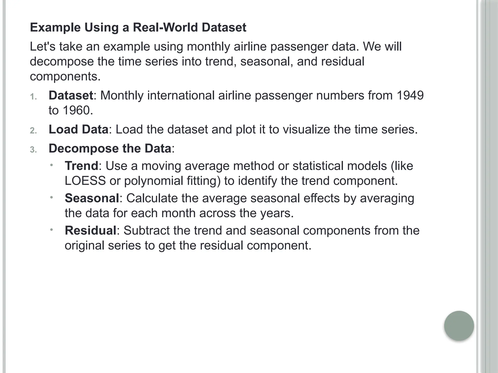
Example Using a Real-World Dataset
Let's take an example using monthly airline passenger data. We will
decompose the time series into trend, seasonal, and residual
components.
1. Dataset: Monthly international airline passenger numbers from 1949
to 1960.
2. Load Data: Load the dataset and plot it to visualize the time series.
3. Decompose the Data:
• Trend: Use a moving average method or statistical models (like
LOESS or polynomial fitting) to identify the trend component.
• Seasonal: Calculate the average seasonal effects by averaging
the data for each month across the years.
• Residual: Subtract the trend and seasonal components from the
original series to get the residual component.
Python Example with statsmodels
Here's a simple Python example using the statsmodels library to
decompose a time series:
import pandas as pd
import matplotlib.pyplot as plt
from statsmodels.tsa.seasonal import seasonal_decompose
# Load the dataset (example with airline passengers)
data = pd.read_csv('airline_passengers.csv', parse_dates=['Month'],
index_col='Month')
# Perform seasonal decomposition
decomposition = seasonal_decompose(data['Passengers'],
model='additive')
# Plot the decomposed components
plt.figure(figsize=(12, 8))
plt.subplot(4, 1, 1)
plt.plot(data['Passengers'], label='Original')
plt.legend(loc='best')
plt.title('Original Series')
plt.subplot(4, 1, 2)
plt.plot(decomposition.trend, label='Trend')
plt.legend(loc='best')
plt.title('Trend Component')
plt.subplot(4, 1, 3)
plt.plot(decomposition.seasonal, label='Seasonal')
plt.legend(loc='best')
plt.title('Seasonal Component')
plt.subplot(4, 1, 4)
plt.plot(decomposition.resid, label='Residual')
plt.legend(loc='best')
plt.title('Residual Component')
plt.tight_layout()
plt.show()
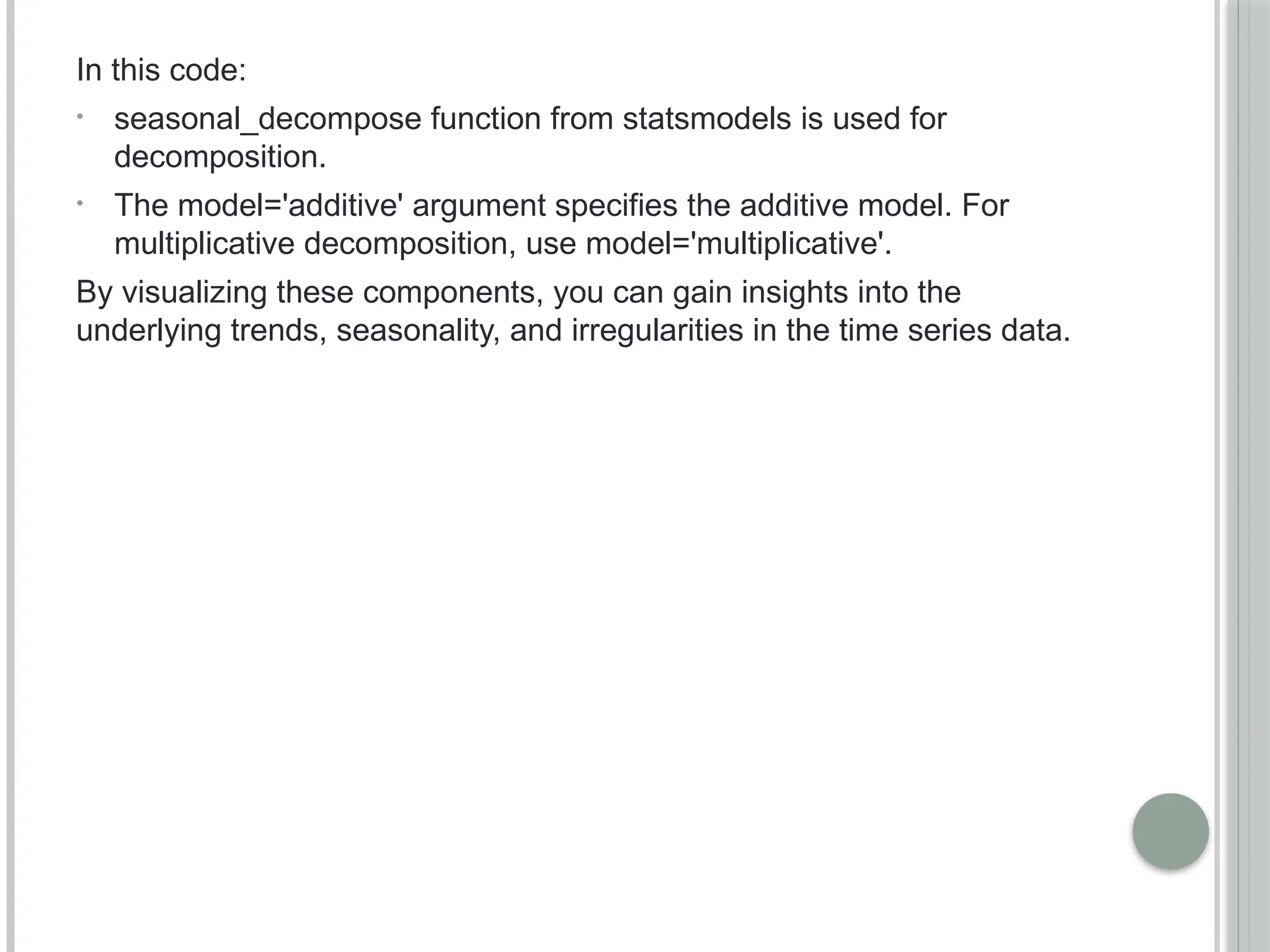
In this code:
• seasonal_decompose function from statsmodels is used for
decomposition.
• The model='additive' argument specifies the additive model. For
multiplicative decomposition, use model='multiplicative'.
By visualizing these components, you can gain insights into the
underlying trends, seasonality, and irregularities in the time series data.
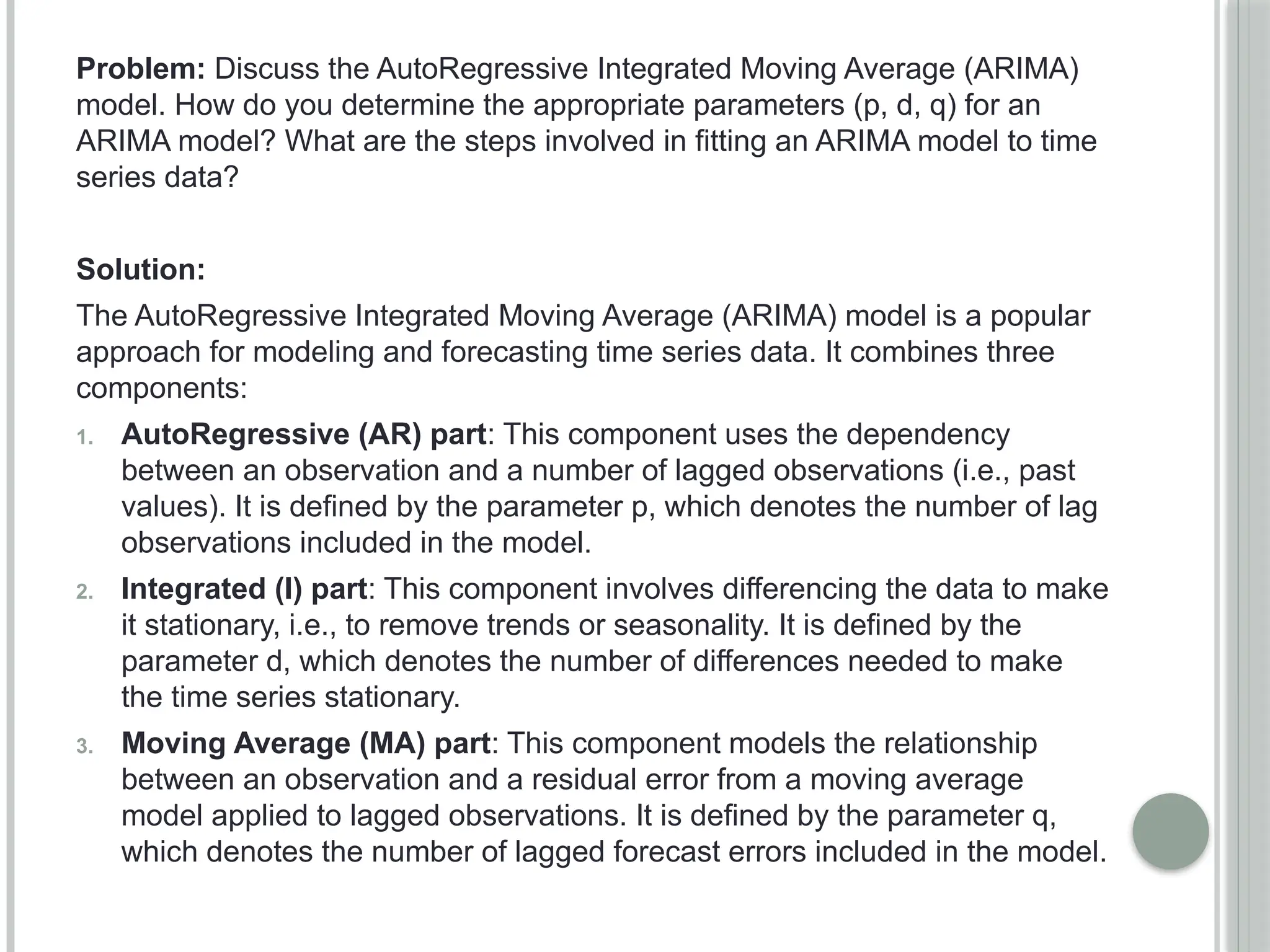
Problem: Discuss the AutoRegressive Integrated Moving Average (ARIMA)
model. How do you determine the appropriate parameters (p, d, q) for an
ARIMA model? What are the steps involved in fitting an ARIMA model to time
series data?
Solution:
The AutoRegressive Integrated Moving Average (ARIMA) model is a popular
approach for modeling and forecasting time series data. It combines three
components:
1. AutoRegressive (AR) part: This component uses the dependency
between an observation and a number of lagged observations (i.e., past
values). It is defined by the parameter p, which denotes the number of lag
observations included in the model.
2. Integrated (I) part: This component involves differencing the data to make
it stationary, i.e., to remove trends or seasonality. It is defined by the
parameter d, which denotes the number of differences needed to make
the time series stationary.
3. Moving Average (MA) part: This component models the relationship
between an observation and a residual error from a moving average
model applied to lagged observations. It is defined by the parameter q,
which denotes the number of lagged forecast errors included in the model.
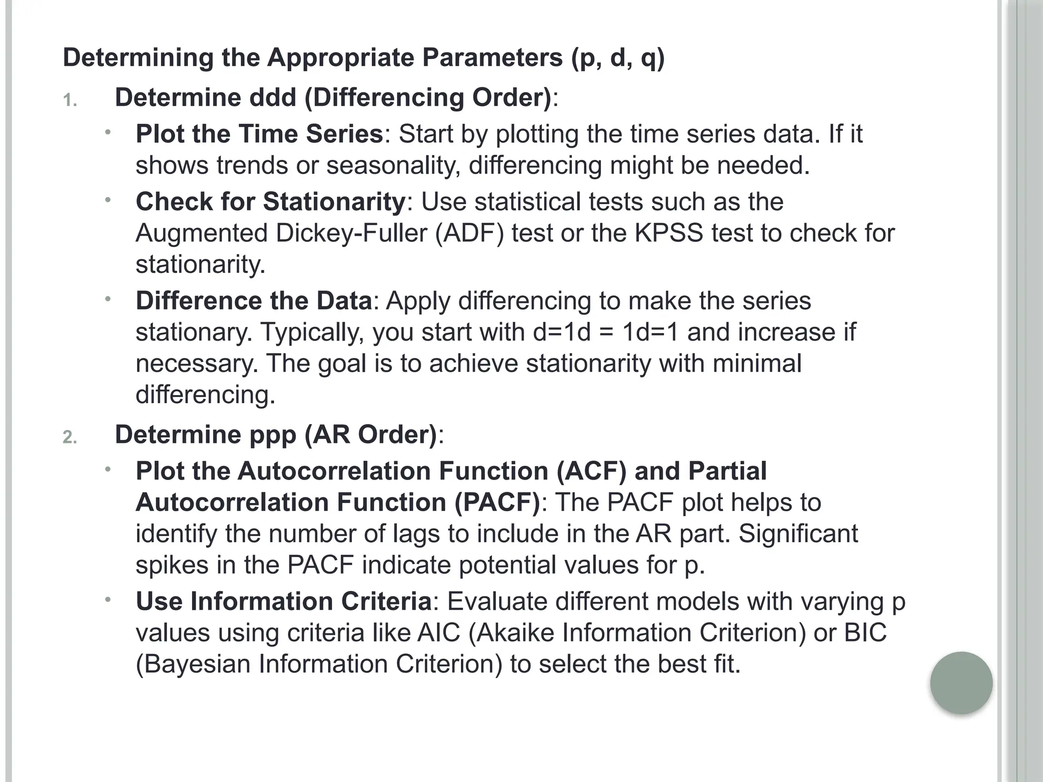
Determining the Appropriate Parameters (p, d, q)
1. Determine ddd (Differencing Order):
• Plot the Time Series: Start by plotting the time series data. If it
shows trends or seasonality, differencing might be needed.
• Check for Stationarity: Use statistical tests such as the
Augmented Dickey-Fuller (ADF) test or the KPSS test to check for
stationarity.
• Difference the Data: Apply differencing to make the series
stationary. Typically, you start with d=1d = 1d=1 and increase if
necessary. The goal is to achieve stationarity with minimal
differencing.
2. Determine ppp (AR Order):
• Plot the Autocorrelation Function (ACF) and Partial
Autocorrelation Function (PACF): The PACF plot helps to
identify the number of lags to include in the AR part. Significant
spikes in the PACF indicate potential values for p.
• Use Information Criteria: Evaluate different models with varying p
values using criteria like AIC (Akaike Information Criterion) or BIC
(Bayesian Information Criterion) to select the best fit.
3. Determine q (MA Order):
• Examine the ACF Plot: The ACF plot shows the correlation of the
series with its lags. Significant spikes in the ACF indicate potential
values for q.
• Use Information Criteria: Similar to p, evaluate different models
with varying q values using AIC or BIC to find the optimal value.
Steps Involved in Fitting an ARIMA Model
4. Preprocessing:
• Plot the Data: Visualize the time series to understand its structure.
• Check Stationarity: Use statistical tests to assess stationarity.
Apply differencing if necessary.
5. Identify Initial Parameters:
• Use ACF and PACF Plots: Analyze these plots to get initial
guesses for p and q.
• Set d: Based on the differencing needed to achieve stationarity.
3. Estimate the Model:
• Fit Models with Different (p, d, q) Combinations: Use statistical
software to fit ARIMA models with various parameter combinations.
• Compare Models: Use AIC, BIC, and other criteria to evaluate and
select the best model.
4. Validate the Model:
• Check Residuals: Analyze the residuals of the fitted model to ensure
they resemble white noise (i.e., they are random and uncorrelated).
• Conduct Forecasting: Use the model to make forecasts and compare
them against actual data.
5. Refine the Model:
• Reassess Parameters: If necessary, adjust p, d, and q based on model
performance and re-evaluate.
6. Implement the Model:
• Deploy for Forecasting: Once satisfied with the model's performance,
use it for making forecasts and apply it to the decision-making process.
Fitting an ARIMA model involves a blend of exploratory data
analysis, statistical testing, and model validation to ensure it
captures the underlying patterns of the time series data effectively.
Problem:
Compare and contrast Long Short-Term Memory (LSTM) networks with
traditional time series models like ARIMA. How do LSTMs address the
issue of vanishing gradients in long sequences?
Solution:
LSTM Networks vs. Traditional Time Series Models
1. Long Short-Term Memory (LSTM) Networks:
 Nature: LSTMs are a type of recurrent neural network (RNN) designed
to handle sequences and time-series data. They are particularly good
at learning and remembering patterns over long sequences.
 Architecture: LSTMs have a specialized architecture with memory
cells and gating mechanisms (input, output, and forget gates) that
regulate the flow of information. This architecture helps the network to
retain information over long periods and manage dependencies in the
data.
 Strengths:
 Handling Long Sequences: LSTMs can manage long-range
dependencies and sequences, which makes them suitable for
tasks like speech recognition, language modeling, and complex
time series forecasting.
 Adaptability: They can learn complex, non-linear relationships in
data without needing extensive feature engineering.
 Vanishing Gradient Problem: LSTMs mitigate the vanishing gradient
problem, which is common in traditional RNNs. This issue occurs when
gradients used in training become very small, effectively stopping the
network from learning long-range dependencies. LSTMs address this
problem with their gating mechanisms and memory cells, which help
preserve gradients over long sequences.
2. Traditional Time Series Models (e.g., ARIMA):
 Nature: ARIMA (AutoRegressive Integrated Moving Average) is a
statistical model used for time series forecasting. It relies on linear
relationships between past values and errors.
 Architecture: ARIMA models are based on autoregression,
differencing, and moving averages. They require careful tuning of
parameters and assumptions about stationarity and linearity in the
data.
 Strengths:
 Interpretability: ARIMA models are relatively straightforward and
offer interpretable results with clear parameters.
 Well-Established: They have been used for many years and are
well understood in the context of classical time series analysis.
 Limitations:
 Linear Assumptions: ARIMA models assume linear relationships,
which may not capture complex patterns in the data.
 Limited Memory: They typically use a fixed window of past
observations and do not inherently capture long-term
dependencies or trends beyond this window.
Addressing Vanishing Gradients in LSTMs
 The vanishing gradient problem arises when gradients used in training
become very small, leading to ineffective learning in long sequences.
LSTMs address this through:
 Memory Cells: They maintain long-term memory through memory
cells that can retain information over many time steps. These cells can
store values for long durations, thus preserving important information.
 Gating Mechanisms: The input, output, and forget gates control the
flow of information. Specifically:
 Input Gate: Controls how much of the new information should be
added to the memory cell.
 Forget Gate: Decides what information should be discarded from
the memory cell.
 Output Gate: Determines what part of the memory cell should be
output.
Problem:
What are some common feature engineering techniques used in time
series forecasting? How can you incorporate external variables
(exogenous variables) into a time series model?
Solution:
Time series forecasting involves predicting future values based on past
observations, and feature engineering can greatly enhance the
performance of your model. Here are some common feature engineering
techniques used in time series forecasting:
Common Feature Engineering Techniques:
• Lag Features: Create features based on past values of the time
series. For example, if you're predicting sales for the next day, you
might include sales data from the previous day or several days ago as
features.
• Rolling Statistics: Compute rolling (or moving) statistics such as
rolling means, rolling variances, or rolling sums. These can help
capture trends and seasonality in the data.
• Seasonal Decomposition: Decompose the time series into seasonal,
trend, and residual components. Features derived from these
components can be useful for capturing underlying patterns.
• Time-Based Features: Include features such as day of the week,
month, quarter, year, and holidays. These can capture seasonality and
cyclical patterns.
• Lagged Differences: Calculate differences between consecutive
observations or between the current observation and a lagged
observation. This can help with stationarity.
• Fourier Transforms: Use Fourier transforms to capture cyclical
patterns and periodicities in the time series.
• Exponential Smoothing: Use exponentially smoothed values as
features. This technique can help in capturing trends and reducing
noise.
• Windowed Features: Create features based on a window of past
observations, such as the mean or median of the last NNN periods.
Incorporating External Variables (Exogenous Variables):
External variables, or exogenous variables, are factors outside the
primary time series that might influence it. Incorporating them can
improve forecasting accuracy. Here’s how you can include exogenous
variables in a time series model:
1. Direct Inclusion: Add exogenous variables as additional features in
your model. For example, if you’re forecasting sales, you might
include advertising spend or economic indicators as features.
2. Regression Models: Use models like ARIMAX (AutoRegressive
Integrated Moving Average with Exogenous Regressors) or SARIMAX
(Seasonal ARIMAX) that explicitly incorporate exogenous variables
alongside the time series data.
3. Feature Engineering for Exogenous Variables: Just like with time
series features, you can engineer features from exogenous variables,
such as lagged values, rolling statistics, or interactions with the
primary time series.
4. External Data Integration: Merge external datasets with your time
series data based on timestamps. For instance, you might incorporate
weather data or demographic information that could impact your time
series.
5. Transfer Function Models: Use transfer function models to model
the relationship between the time series and the external variables.
These models help in understanding how external variables affect the
time series over time.
6. Feature Selection: Use techniques like correlation analysis or feature
importance from machine learning models to select the most relevant
exogenous variables.
Problem:
Describe the differences between traditional cross-validation and time
series cross-validation. What are the key considerations when applying
cross-validation to time series data?
Solution:
Cross-validation is a technique used to evaluate the performance of a
model by partitioning the data into subsets and training/testing the model
on these subsets. The traditional cross-validation approach and time
series cross-validation differ mainly in how they handle the temporal
nature of time series data. Here are the key differences and
considerations:
Traditional Cross-Validation
• Data Partitioning: Traditional cross-validation typically involves
randomly splitting the dataset into multiple folds (e.g., k-fold cross-
validation). Each fold is used once as a test set while the remaining
folds are used for training. This method assumes that data points are
independent of each other.
• Assumption: It assumes that the data is independent and identically
distributed (i.i.d.), meaning that the data points do not have any
inherent order or temporal structure.
• Shuffling: In traditional cross-validation, data points can be shuffled or
randomly sampled to create training and testing sets, which helps
ensure that the model is evaluated on a representative subset of the
data.
Time Series Cross-Validation
• Data Partitioning: In time series cross-validation, the data is split in a
way that respects the temporal order of observations. Common
approaches include:
• Rolling Window: The training set is a rolling window of fixed size
that moves forward in time, with the test set being the subsequent
period.
• Expanding Window: The training set starts from the beginning
and expands over time, with the test set being the next period.
• Assumption: Time series cross-validation acknowledges the temporal
dependencies between observations. The model needs to be
evaluated in a way that respects these dependencies and mimics real-
world scenarios where future data points are used for prediction based
on past data.
• Shuffling: Shuffling data is generally not appropriate for time series
cross-validation because it would violate the temporal order of
observations.
Key Considerations for Time Series Cross-Validation
• Temporal Order: Ensure that the validation process respects the time
ordering of data. The training set must always come before the test set
to simulate how models would be used in practice.
• Seasonality and Trends: Consider any seasonality or trends present
in the data. Cross-validation should account for these patterns to
provide a realistic assessment of model performance.
• Data Leakage: Avoid data leakage by ensuring that information from
the future does not influence the model training. This is crucial for time
series data where future values should not be used to predict past or
present values.
• Stationarity: For some time series models, ensuring stationarity
(constant statistical properties over time) might be necessary. The
cross-validation strategy should account for changes in the data's
statistical properties over time.
By respecting the temporal structure and dependencies inherent in time
series data, time series cross-validation provides a more accurate
assessment of a model's performance in practical, real-world scenarios.
CONCLUSION
In this assignment, we explored the concept of seasonal decomposition
of time series data, breaking it down into its trend, seasonal, and
residual components. Through the practical application to a real-world
dataset, we gained insights into how these components can be isolated
to better understand the underlying patterns and irregularities in the
data. This technique is invaluable for making informed predictions and
decisions based on historical data trends. For further assistance and
detailed explanations, Programming Homework Help offers
comprehensive support and expert solutions to enhance your learning
experience in data analysis and programming.
For any assignment-related queries, you can contact us at:
• Email: support@programminghomeworkhelp.com
• Website: https://www.programminghomeworkhelp.com/

Seasonal Decomposition of Time Series Data

  • 1.
    SEASONAL DECOMPOSITION OF TIME SERIESDATA IN MACHINE LEARNING Decomposing Time Series into Trend, Seasonal, and Residual Components using Real-World Data For Any Assignment Related Queries Reach Us At: Email: - support@programminghomeworkhelp.com or Website: - https://www.programminghomeworkhelp.com/
  • 2.
    SEASONAL DECOMPOSITION OF TIMESERIES DATA Welcome to the sample assignment from programminghomeworkhelp.com where we simplify Seasonal decomposition of time series data is a fundamental technique in time series analysis, used to understand and interpret the underlying patterns in datasets. This method involves breaking down a series into three main components: trend, seasonal, and residual. By doing so, it helps to isolate long-term movements, recurring patterns, and irregular variations. In this assignment, we will explore these concepts and apply them to a real-world dataset. For additional support and resources, Programming Homework Help provides expert guidance and solutions tailored to various programming and data analysis challenges.
  • 3.
    Problem: Explain the conceptof seasonal decomposition of time series data. How would you decompose a time series into its trend, seasonal, and residual components? Provide an example using a real-world dataset. Solution: Seasonal decomposition of time series data is a technique used to analyze and understand the underlying patterns in a time series dataset. This process breaks down the data into three main components: • Trend: This represents the long-term progression or movement in the data. It's the general direction in which the data is moving over an extended period. • Seasonal: This captures regular, repeating patterns or fluctuations within specific time intervals, such as daily, monthly, or yearly. These patterns often result from external factors that influence the data at consistent intervals. • Residual: This is the remaining variation in the data after removing the trend and seasonal components. It represents the irregular or random noise in the data that cannot be attributed to the trend or seasonal effects.
  • 4.
    Steps for Decomposition 1.Determine the Decomposition Method: The two primary methods for decomposition are: • Additive Decomposition: Used when the seasonal variations are roughly constant throughout the series. • Multiplicative Decomposition: Used when the seasonal variations are proportional to the level of the series. 2. Extract Trend Component: Smooth the data to identify the underlying trend. This can be done using moving averages or other smoothing techniques. 3. Remove Trend and Extract Seasonal Component: Subtract the trend component from the original data to isolate the seasonal component. Calculate the average seasonal effects over the seasonality period. 4. Identify Residual Component: Subtract both the trend and seasonal components from the original data to obtain the residuals.
  • 5.
    Example Using aReal-World Dataset Let's take an example using monthly airline passenger data. We will decompose the time series into trend, seasonal, and residual components. 1. Dataset: Monthly international airline passenger numbers from 1949 to 1960. 2. Load Data: Load the dataset and plot it to visualize the time series. 3. Decompose the Data: • Trend: Use a moving average method or statistical models (like LOESS or polynomial fitting) to identify the trend component. • Seasonal: Calculate the average seasonal effects by averaging the data for each month across the years. • Residual: Subtract the trend and seasonal components from the original series to get the residual component.
  • 6.
    Python Example withstatsmodels Here's a simple Python example using the statsmodels library to decompose a time series: import pandas as pd import matplotlib.pyplot as plt from statsmodels.tsa.seasonal import seasonal_decompose # Load the dataset (example with airline passengers) data = pd.read_csv('airline_passengers.csv', parse_dates=['Month'], index_col='Month') # Perform seasonal decomposition decomposition = seasonal_decompose(data['Passengers'], model='additive') # Plot the decomposed components plt.figure(figsize=(12, 8))
  • 7.
    plt.subplot(4, 1, 1) plt.plot(data['Passengers'],label='Original') plt.legend(loc='best') plt.title('Original Series') plt.subplot(4, 1, 2) plt.plot(decomposition.trend, label='Trend') plt.legend(loc='best') plt.title('Trend Component') plt.subplot(4, 1, 3) plt.plot(decomposition.seasonal, label='Seasonal') plt.legend(loc='best') plt.title('Seasonal Component') plt.subplot(4, 1, 4) plt.plot(decomposition.resid, label='Residual') plt.legend(loc='best') plt.title('Residual Component') plt.tight_layout() plt.show()
  • 8.
    In this code: •seasonal_decompose function from statsmodels is used for decomposition. • The model='additive' argument specifies the additive model. For multiplicative decomposition, use model='multiplicative'. By visualizing these components, you can gain insights into the underlying trends, seasonality, and irregularities in the time series data.
  • 9.
    Problem: Discuss theAutoRegressive Integrated Moving Average (ARIMA) model. How do you determine the appropriate parameters (p, d, q) for an ARIMA model? What are the steps involved in fitting an ARIMA model to time series data? Solution: The AutoRegressive Integrated Moving Average (ARIMA) model is a popular approach for modeling and forecasting time series data. It combines three components: 1. AutoRegressive (AR) part: This component uses the dependency between an observation and a number of lagged observations (i.e., past values). It is defined by the parameter p, which denotes the number of lag observations included in the model. 2. Integrated (I) part: This component involves differencing the data to make it stationary, i.e., to remove trends or seasonality. It is defined by the parameter d, which denotes the number of differences needed to make the time series stationary. 3. Moving Average (MA) part: This component models the relationship between an observation and a residual error from a moving average model applied to lagged observations. It is defined by the parameter q, which denotes the number of lagged forecast errors included in the model.
  • 10.
    Determining the AppropriateParameters (p, d, q) 1. Determine ddd (Differencing Order): • Plot the Time Series: Start by plotting the time series data. If it shows trends or seasonality, differencing might be needed. • Check for Stationarity: Use statistical tests such as the Augmented Dickey-Fuller (ADF) test or the KPSS test to check for stationarity. • Difference the Data: Apply differencing to make the series stationary. Typically, you start with d=1d = 1d=1 and increase if necessary. The goal is to achieve stationarity with minimal differencing. 2. Determine ppp (AR Order): • Plot the Autocorrelation Function (ACF) and Partial Autocorrelation Function (PACF): The PACF plot helps to identify the number of lags to include in the AR part. Significant spikes in the PACF indicate potential values for p. • Use Information Criteria: Evaluate different models with varying p values using criteria like AIC (Akaike Information Criterion) or BIC (Bayesian Information Criterion) to select the best fit.
  • 11.
    3. Determine q(MA Order): • Examine the ACF Plot: The ACF plot shows the correlation of the series with its lags. Significant spikes in the ACF indicate potential values for q. • Use Information Criteria: Similar to p, evaluate different models with varying q values using AIC or BIC to find the optimal value. Steps Involved in Fitting an ARIMA Model 4. Preprocessing: • Plot the Data: Visualize the time series to understand its structure. • Check Stationarity: Use statistical tests to assess stationarity. Apply differencing if necessary. 5. Identify Initial Parameters: • Use ACF and PACF Plots: Analyze these plots to get initial guesses for p and q. • Set d: Based on the differencing needed to achieve stationarity.
  • 12.
    3. Estimate theModel: • Fit Models with Different (p, d, q) Combinations: Use statistical software to fit ARIMA models with various parameter combinations. • Compare Models: Use AIC, BIC, and other criteria to evaluate and select the best model. 4. Validate the Model: • Check Residuals: Analyze the residuals of the fitted model to ensure they resemble white noise (i.e., they are random and uncorrelated). • Conduct Forecasting: Use the model to make forecasts and compare them against actual data. 5. Refine the Model: • Reassess Parameters: If necessary, adjust p, d, and q based on model performance and re-evaluate. 6. Implement the Model: • Deploy for Forecasting: Once satisfied with the model's performance, use it for making forecasts and apply it to the decision-making process. Fitting an ARIMA model involves a blend of exploratory data analysis, statistical testing, and model validation to ensure it captures the underlying patterns of the time series data effectively.
  • 13.
    Problem: Compare and contrastLong Short-Term Memory (LSTM) networks with traditional time series models like ARIMA. How do LSTMs address the issue of vanishing gradients in long sequences? Solution: LSTM Networks vs. Traditional Time Series Models 1. Long Short-Term Memory (LSTM) Networks:  Nature: LSTMs are a type of recurrent neural network (RNN) designed to handle sequences and time-series data. They are particularly good at learning and remembering patterns over long sequences.  Architecture: LSTMs have a specialized architecture with memory cells and gating mechanisms (input, output, and forget gates) that regulate the flow of information. This architecture helps the network to retain information over long periods and manage dependencies in the data.  Strengths:  Handling Long Sequences: LSTMs can manage long-range dependencies and sequences, which makes them suitable for tasks like speech recognition, language modeling, and complex time series forecasting.
  • 14.
     Adaptability: Theycan learn complex, non-linear relationships in data without needing extensive feature engineering.  Vanishing Gradient Problem: LSTMs mitigate the vanishing gradient problem, which is common in traditional RNNs. This issue occurs when gradients used in training become very small, effectively stopping the network from learning long-range dependencies. LSTMs address this problem with their gating mechanisms and memory cells, which help preserve gradients over long sequences. 2. Traditional Time Series Models (e.g., ARIMA):  Nature: ARIMA (AutoRegressive Integrated Moving Average) is a statistical model used for time series forecasting. It relies on linear relationships between past values and errors.  Architecture: ARIMA models are based on autoregression, differencing, and moving averages. They require careful tuning of parameters and assumptions about stationarity and linearity in the data.  Strengths:  Interpretability: ARIMA models are relatively straightforward and offer interpretable results with clear parameters.  Well-Established: They have been used for many years and are well understood in the context of classical time series analysis.
  • 15.
     Limitations:  LinearAssumptions: ARIMA models assume linear relationships, which may not capture complex patterns in the data.  Limited Memory: They typically use a fixed window of past observations and do not inherently capture long-term dependencies or trends beyond this window. Addressing Vanishing Gradients in LSTMs  The vanishing gradient problem arises when gradients used in training become very small, leading to ineffective learning in long sequences. LSTMs address this through:  Memory Cells: They maintain long-term memory through memory cells that can retain information over many time steps. These cells can store values for long durations, thus preserving important information.  Gating Mechanisms: The input, output, and forget gates control the flow of information. Specifically:  Input Gate: Controls how much of the new information should be added to the memory cell.  Forget Gate: Decides what information should be discarded from the memory cell.  Output Gate: Determines what part of the memory cell should be output.
  • 16.
    Problem: What are somecommon feature engineering techniques used in time series forecasting? How can you incorporate external variables (exogenous variables) into a time series model? Solution: Time series forecasting involves predicting future values based on past observations, and feature engineering can greatly enhance the performance of your model. Here are some common feature engineering techniques used in time series forecasting: Common Feature Engineering Techniques: • Lag Features: Create features based on past values of the time series. For example, if you're predicting sales for the next day, you might include sales data from the previous day or several days ago as features. • Rolling Statistics: Compute rolling (or moving) statistics such as rolling means, rolling variances, or rolling sums. These can help capture trends and seasonality in the data. • Seasonal Decomposition: Decompose the time series into seasonal, trend, and residual components. Features derived from these components can be useful for capturing underlying patterns.
  • 17.
    • Time-Based Features:Include features such as day of the week, month, quarter, year, and holidays. These can capture seasonality and cyclical patterns. • Lagged Differences: Calculate differences between consecutive observations or between the current observation and a lagged observation. This can help with stationarity. • Fourier Transforms: Use Fourier transforms to capture cyclical patterns and periodicities in the time series. • Exponential Smoothing: Use exponentially smoothed values as features. This technique can help in capturing trends and reducing noise. • Windowed Features: Create features based on a window of past observations, such as the mean or median of the last NNN periods. Incorporating External Variables (Exogenous Variables): External variables, or exogenous variables, are factors outside the primary time series that might influence it. Incorporating them can improve forecasting accuracy. Here’s how you can include exogenous variables in a time series model:
  • 18.
    1. Direct Inclusion:Add exogenous variables as additional features in your model. For example, if you’re forecasting sales, you might include advertising spend or economic indicators as features. 2. Regression Models: Use models like ARIMAX (AutoRegressive Integrated Moving Average with Exogenous Regressors) or SARIMAX (Seasonal ARIMAX) that explicitly incorporate exogenous variables alongside the time series data. 3. Feature Engineering for Exogenous Variables: Just like with time series features, you can engineer features from exogenous variables, such as lagged values, rolling statistics, or interactions with the primary time series. 4. External Data Integration: Merge external datasets with your time series data based on timestamps. For instance, you might incorporate weather data or demographic information that could impact your time series. 5. Transfer Function Models: Use transfer function models to model the relationship between the time series and the external variables. These models help in understanding how external variables affect the time series over time. 6. Feature Selection: Use techniques like correlation analysis or feature importance from machine learning models to select the most relevant exogenous variables.
  • 19.
    Problem: Describe the differencesbetween traditional cross-validation and time series cross-validation. What are the key considerations when applying cross-validation to time series data? Solution: Cross-validation is a technique used to evaluate the performance of a model by partitioning the data into subsets and training/testing the model on these subsets. The traditional cross-validation approach and time series cross-validation differ mainly in how they handle the temporal nature of time series data. Here are the key differences and considerations: Traditional Cross-Validation • Data Partitioning: Traditional cross-validation typically involves randomly splitting the dataset into multiple folds (e.g., k-fold cross- validation). Each fold is used once as a test set while the remaining folds are used for training. This method assumes that data points are independent of each other. • Assumption: It assumes that the data is independent and identically distributed (i.i.d.), meaning that the data points do not have any inherent order or temporal structure.
  • 20.
    • Shuffling: Intraditional cross-validation, data points can be shuffled or randomly sampled to create training and testing sets, which helps ensure that the model is evaluated on a representative subset of the data. Time Series Cross-Validation • Data Partitioning: In time series cross-validation, the data is split in a way that respects the temporal order of observations. Common approaches include: • Rolling Window: The training set is a rolling window of fixed size that moves forward in time, with the test set being the subsequent period. • Expanding Window: The training set starts from the beginning and expands over time, with the test set being the next period. • Assumption: Time series cross-validation acknowledges the temporal dependencies between observations. The model needs to be evaluated in a way that respects these dependencies and mimics real- world scenarios where future data points are used for prediction based on past data. • Shuffling: Shuffling data is generally not appropriate for time series cross-validation because it would violate the temporal order of observations.
  • 21.
    Key Considerations forTime Series Cross-Validation • Temporal Order: Ensure that the validation process respects the time ordering of data. The training set must always come before the test set to simulate how models would be used in practice. • Seasonality and Trends: Consider any seasonality or trends present in the data. Cross-validation should account for these patterns to provide a realistic assessment of model performance. • Data Leakage: Avoid data leakage by ensuring that information from the future does not influence the model training. This is crucial for time series data where future values should not be used to predict past or present values. • Stationarity: For some time series models, ensuring stationarity (constant statistical properties over time) might be necessary. The cross-validation strategy should account for changes in the data's statistical properties over time. By respecting the temporal structure and dependencies inherent in time series data, time series cross-validation provides a more accurate assessment of a model's performance in practical, real-world scenarios.
  • 22.
    CONCLUSION In this assignment,we explored the concept of seasonal decomposition of time series data, breaking it down into its trend, seasonal, and residual components. Through the practical application to a real-world dataset, we gained insights into how these components can be isolated to better understand the underlying patterns and irregularities in the data. This technique is invaluable for making informed predictions and decisions based on historical data trends. For further assistance and detailed explanations, Programming Homework Help offers comprehensive support and expert solutions to enhance your learning experience in data analysis and programming. For any assignment-related queries, you can contact us at: • Email: support@programminghomeworkhelp.com • Website: https://www.programminghomeworkhelp.com/