Time series analysis 101

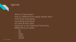
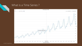
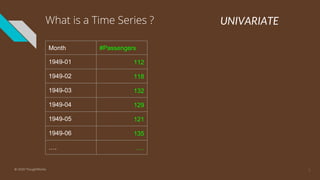
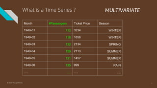
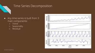
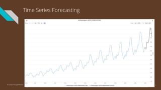
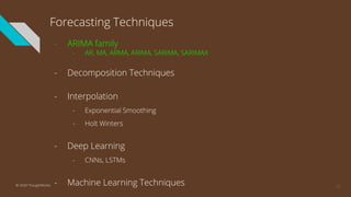
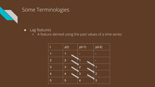
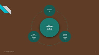
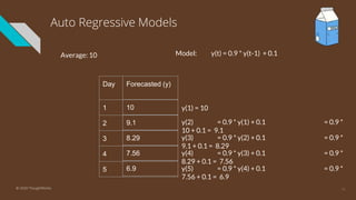
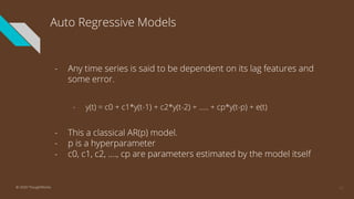
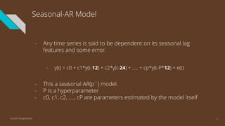
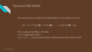
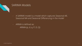
1
Time Series Analysis 101
- Tarun Abichandani
© 2020 ThoughtWorks

Agenda
- What is a Time Series?
- How is it different from regular tabular data ?
- Time Series Forecasting
- Forecasting Techniques
- ACF plots & PACF plots
- Stationary vs Non Stationary Time Series
- ARIMA family of models
- AR,
- MA,
- ARMA,
- ARIMA,
- SARIMA
2© 2020 ThoughtWorks

Before we start,
● The aim of this talk is to get you a introduced to Time Series
Analysis and get into the details of ARIMA set of models.
● Although we will cover everything from the basics, context of
what a ML model is, would be useful.
● Everything is linked.
● For simplicity, some concepts have been abstracted.

What is a Time Series ?

Month #Passengers
1949-01 112
1949-02 118
1949-03 132
1949-04 129
1949-05 121
1949-06 135
…. ….
UNIVARIATE

Month #Passengers
1949-01 112
1949-02 118
1949-03 132
1949-04 129
1949-05 121
1949-06 135
…. ….
Ticket Price Season
3234 WINTER
1656 WINTER
2134 SPRING
2113 SUMMER
1457 SUMMER
999 RAIN
…. ….
MULTIVARIATE

Time Series Decomposition
● Any time series is built from 3
main components:
○ Trend
○ Seasonality
○ Residual

Time Series Forecasting

Examples of Time Series Forecasting
● Forecasting the corn yield in tons by state each year.
● Forecasting the closing price of a stock each day.
● Forecasting the birth rate at all hospitals in a city each year.
● Forecasting product sales in units sold each day for a store.
● Forecasting the number of passengers through a train station
each day.
● Forecasting unemployment for a state each quarter.
● Forecasting utilization demand on a server each hour.
● Forecasting the average price of gasoline in a city each day.
It is not a silver bullet

Prediction vs Forecasting
Area Locality Age Number of
Rooms
Price
3000 NEAR SEA 5 4 452600
2556 CITY 10 3 358500
3223 CITY 20 3 352100
2332 SUBURB 20 2 341300
3432 CITY 4 3 342200
2123 NEAR SEA 16 2 269700
…. …. …. …. ….

Prediction vs Forecasting
Month Season
1949-01 WINTER
1949-02 WINTER
1949-03 SPRING
1949-04 SUMMER
1949-05 SUMMER
1949-06 RAIN
…. ….
Ticket Price #Passengers
3234 112
1656 118
2134 132
2113 129
1457 121
999 135
…. ….

Forecasting Techniques
- ARIMA family
- AR, MA, ARMA, ARIMA, SARIMA, SARIMAX
- Decomposition Techniques
- Interpolation
- Exponential Smoothing
- Holt Winters
- Deep Learning
- CNNs, LSTMs
- Machine Learning Techniques 12© 2020 ThoughtWorks

ARIMA Family

Some Terminologies
● Lag features
○ A feature derived using the past values of a time series
t y(t)
1 1
2 2
3 3
4 4
5 5
y(t-2)
-
-
1
2
3
y(t-1)
-
1
2
3
4

ARIMA
(p,d,q)
Integrated
(d)
Auto
Regressive
models
(p)
Moving
Average
models
(q)

Auto Regressive Models
Day Forecasted (y)
1
2
3
4
5
Average: 10 Model: y(t) = 0.9 * y(t-1) + 0.1
10
9.1
8.29
7.56
6.9
y(1) = 10
y(2) = 0.9 * y(1) + 0.1 = 0.9 *
10 + 0.1 = 9.1
y(3) = 0.9 * y(2) + 0.1 = 0.9 *
9.1 + 0.1 = 8.29
y(4) = 0.9 * y(3) + 0.1 = 0.9 *
8.29 + 0.1 = 7.56
y(5) = 0.9 * y(4) + 0.1 = 0.9 *
7.56 + 0.1 = 6.9

Auto Regressive Models
- Any time series is said to be dependent on its lag features and
some error.
- y(t) = c0 + c1*y(t-1) + c2*y(t-2) + ….. + cp*y(t-p) + e(t)
- This a classical AR(p) model.
- p is a hyperparameter
- c0, c1, c2, …., cp are parameters estimated by the model itself

How to calculate ‘p’ ? | Autocorrelation Plot
Autocorrelation plot : Plot of k vs corr(y(t), y(t-k))
y
...
6
8
10
12
14
y(t-2) y(t-3)
... ...
2 0
4 2
6 4
8 6
10 8
y(t-1)
...
4
6
8
10
12
Corr 0.8 0.604 0.414

How to calculate ‘p’ ? | Partial Autocorrelation Plot
y
...
2
4
6
8
6
y(t-2) y(t-3)
... ...
2 0
4 2
6 4
8 6
10 8
y(t-1)
...
4
6
8
10
12
Corr 0.8 -0.101 -0.102

Lets try it
p = 2

Moving Average Models
Day Forecasted (y) Delta (e) Actual
1
2
3
4
5
Average: 10 Model: y(t) = Avg + 0.5 * e(t-1)
10 -2 8
9 1 10
10.5 0 10.5
10 2 12
11 1 12

- Any time series is said to be dependent on the error of its lag
terms.
- y(t) = c0 + c1*e(t-1) + c2*e(t-2) + ….. + cp*e(t-q)
- This a classical MA(q) model.
- q is a hyperparameter
- c0, c1, c2, …., cq are parameters estimated by the model itself

- Any time series is said to be dependent on the error of its lag
terms.
- y(t) = c0 + c1*e(t-1) + c2*e(t-2) + ….. + cp*e(t-q)
- The value of q is determined using the ACF Plot

Lets try it

Taking a step back : Stationarity
- All of these models assume that the time series should be
stationery
- A stationary time series is one with constant behaviour over
time. This behaviour is defined by:
- Constant Mean
- Constant Variance
- Constant Autocorrelation
- Why ?
- In practice this is not possible, but there are ways to make a
model stationary

Differencing
y(t) y(t-1)
10 -
14 10
16 14
19 16
25 19
y`(t) = y(t) - y(t-1)
-
4
2
3
6

Differencing
- Differencing is one of the ways to convert a non-stationary time
series into a stationary time series
- It simply translates the time series into:
- y’(t) = y(t) - y(t-1) : First Order
differencing
- y’’(t) = y’(t) - y’(t-1) : Second Order
differencing

Differencing Example

Lets try it now
p = 2
q = 2
d = 1

ARMA Models
- Any time series is said to be dependent on the lag features as
well as the error of its lag terms.
- y(t) = c0 + c1*y(t-1) + c2*y(t-2) + ….. + cp*y(t-p) +
c`1*e(t-1) + c`2*e(t-2) + ….. + c`p*e(t-q)
- This a classical ARMA model.
- p, q is a hyperparameter
- c0, c1, c2, …., cp, c`0, c`1, c`2, …., c`q are parameters estimated
by the model itself

ARIMA Models
- Now, one option is that you make your time series stationary
and then feed it to ARMA models.
- ARIMA models on the other take care about this.
- ‘I’ signifies integrated
- It is same as ARMA model with an additional hyper parameter
(d), which signifies how much you want to difference the time
series to make it stationary.
- ARIMA is defined as:
ARIMA (p, d, q)

Lets try it now

Lets try it now
p = 2
q = 2
d = 1

Seasonal Period
- The seasonal period is the time after which a time series repeats a pattern

Seasonal Differencing
- First order: y’(t) = y(t) - y(t-12)
Note: When you give your function this parameter,
you will give a seasonal order as 1

Lets try it now
p = 2
q = 2
d = 1
D = 1

Seasonal-AR Model
- Any time series is said to be dependent on its seasonal lag
features and some error.
- y(t) = c0 + c1*y(t-12) + c2*y(t-24) + ….. + cp*y(t-P*12) + e(t)
- This a seasonal AR(p`) model.
- P is a hyperparameter
- c0, c1, c2, …., cP are parameters estimated by the model itself

Seasonal-MA Model
- Any time series is said to be dependent on its seasonal error.
- y(t) = c0 + c1*e(t-12) + c2*e(t-24) + ….. + cq*e(t-Q*12) + e(t)
- This a seasonal MA(q`) model.
- Q is a hyperparameter
- c0, c1, c2, …., cQ are parameters estimated by the model itself

SARIMA Models
- A SARIMA model is a model which captures Seasonal AR,
Seasonal MA and Seasonal Differencing in the model
- ARIMA is defined as:
ARIMA (p, d, q, P, D, Q)

Lets try it now

Further reading
● https://www.otexts.org/fpp
● https://online.stat.psu.edu/stat510/
● https://www.youtube.com/channel/UCUcpVoi5KkJmnE3bvEhHR0Q

References
● https://www.otexts.org/fpp
● https://online.stat.psu.edu/stat501/lesson/14/14.1
● https://online.stat.psu.edu/stat510/lesson/2/2.1
● https://towardsdatascience.com/stationarity-in-time-series-analysis-90c94f27322
● https://www.youtube.com/channel/UCUcpVoi5KkJmnE3bvEhHR0Q

Thank You
Q&A

Time series analysis 101

More Related Content

What's hot

Similar to Time series analysis 101

More from Balvinder Hira

Recently uploaded

Time series analysis 101

Editor's Notes