The document discusses the ARIMA model (AutoRegressive Integrated Moving Average) and its components, defined as ARIMA(p, d, q), where p, d, and q represent the autoregressive terms, degree of differencing, and moving average terms, respectively. It emphasizes the importance of using stationary time-series data for effective modeling, describing the process of differencing to achieve stationarity and outlining steps for forecasting. The document also mentions the significance of parameters p, d, and q in predicting future values based on past observations and errors.

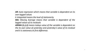
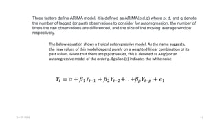
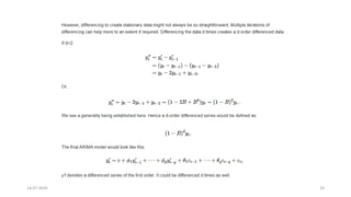
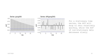
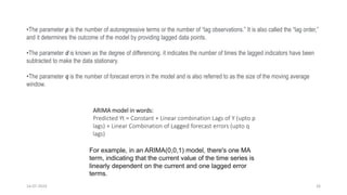
1. APPLIED DATA SCIENCE
ARIMA Model

2. OBJECTIVE
“
“
To demonstrate ARIMA model.

7. 14-07-2024 7

8. 8

9. 9

10. 14-07-2024 10

11. 14-07-2024 11
Three factors define ARIMA model, it is defined as ARIMA(p,d,q) where p, d, and q denote
the number of lagged (or past) observations to consider for autoregression, the number of
times the raw observations are differenced, and the size of the moving average window
respectively.
The below equation shows a typical autoregressive model. As the name suggests,
the new values of this model depend purely on a weighted linear combination of its
past values. Given that there are p past values, this is denoted as AR(p) or an
autoregressive model of the order p. Epsilon (ε) indicates the white noise

12. 14-07-2024 12
Next, the moving average is defined as follows:
the moving average
Here, the future value y(t) is computed based on the errors εt made by
the previous model. So, each successive term looks one step further
into the past to incorporate the mistakes made by that model in the
current computation. Based on the window we are willing to look past,
the value of q is set. Thus, the above model can be independently
denoted as a moving average order q or simply MA(q).
Moving Average (MA) model works by analysing how
wrong you were in predicting values for the previous time-
periods to make a better estimate for the current time-
period.

13. Why does ARIMA need Stationary Time-Series Data?
Stationarity
A stationary time series data is one whose properties do not depend on the time, That is why
time series with trends, or with seasonality, are not stationary. the trend and seasonality will
affect the value of the time series at different times,
A stationary time series is one whose statistical properties such as mean, variance,
autocorrelation, etc. are all constant over time.
On the other hand for stationarity it does not matter when you observe it, it should look
much the same at any point in time. In general, a stationary time series will have no
predictable patterns in the long-term.

14. Why does ARIMA need Stationary Time-Series Data?

15. Why does ARIMA need Stationary Time-Series Data?
Time series data must be made stationary to remove any obvious correlation and collinearity
with the past data.
In stationary time-series data, the properties or value of a sample observation does not depend
on the timestamp at which it is observed. For example, given a hypothetical dataset of the year-
wise population of an area, if one observes that the population increases two-fold each year or
increases by a fixed amount, then this data is non-stationary.
Any given observation is highly dependent on the year since the population value would rely on
how far it is from an arbitrary past year. This dependency can induce incorrect bias while
training a model with time-series data.
To remove this correlation, ARIMA uses differencing to make the data stationary.
Differencing, at its simplest, involves taking the difference of two adjacent data points.

16. 14-07-2024 S.Vairachilai 16

17. 14-07-2024 17
For example, the left graph above shows Google's stock price for 200 days. While the
graph on the right is the differenced version of the first graph – meaning that it shows the
change in Google stock of 200 days. There is a pattern observable in the first graph, and
these trends are a sign of non-stationary time series data. However, no trend or
seasonality, or increasing variance is observed in the second figure. Thus, we can say that
the differenced version is stationary.

18. 14-07-2024 18
This change can simply be modeled by
Where B denotes the backshift operator defined as

19. 14-07-2024 19

20. 14-07-2024 20
Combining all of the three types of models above gives
the resulting ARIMA(p,d,q) model.

21. 14-07-2024 21
In general, it is a good practice to follow the next steps when doing time-series forecasting:
•Step 1 — Check Stationarity: If a time series has a trend or seasonality component, it
must be made stationary.
•Step 2 — Determine the d value: If the time series is not stationary, it needs to be
stationarized through differencing.
•Step 3 — Select AR and MA terms: Use the ACF and PACF to decide whether to include
an AR term, MA term, (or) ARMA.
•Step 4 — Build the model

22. 14-07-2024 22
For a stationary time
series, the ACF will
drop to zero relatively
quickly, while the ACF
of non-stationary data
decreases slowly.

23. 14-07-2024 23
For a stationary time
series, the ACF will
drop to zero relatively
quickly, while the ACF
of non-stationary data
decreases slowly.

24. 14-07-2024 24
The right order of differencing is the minimum differencing required to get a near-
stationary series which roams around a defined mean and the ACF plot reaches to zero
fairly quick.
If the autocorrelations are positive for many number of lags (10 or more), then the
series needs further differencing.
On the other hand, if the lag 1 autocorrelation itself is too negative, then the series is
probably over-differenced

25. 14-07-2024 25
Check if the series is stationary using the Augmented Dickey
Fuller test (adfuller()), from the statsmodels package.
Why?
Because, you need differencing only if the series is non-
stationary. Else, no differencing is needed, that is, d=0.
The null hypothesis of the ADF test is that the time series is
non-stationary. So, if the p-value of the test is less than the
significance level (0.05) then you reject the null hypothesis and
infer that the time series is indeed stationary.
So, in our case, if P Value > 0.05 we go ahead with finding the
order of differencing.

26. 14-07-2024 26
•The parameter p is the number of autoregressive terms or the number of “lag observations.” It is also called the “lag order,”
and it determines the outcome of the model by providing lagged data points.
•The parameter d is known as the degree of differencing. it indicates the number of times the lagged indicators have been
subtracted to make the data stationary.
•The parameter q is the number of forecast errors in the model and is also referred to as the size of the moving average
window.
ARIMA model in words:
Predicted Yt = Constant + Linear combination Lags of Y (upto p
lags) + Linear Combination of Lagged forecast errors (upto q
lags)
For example, in an ARIMA(0,0,1) model, there's one MA
term, indicating that the current value of the time series is
linearly dependent on the current and one lagged error
terms.

27. Thank you