Downloaded 74 times


![Their presence indicates a northern boreal for-est
ecosystem rather than today’s Arctic environ-ment.
Ancient Biomolecules from
Deep Ice Cores Reveal a Forested
Southern Greenland
Eske Willerslev,1* Enrico Cappellini,2 Wouter Boomsma,3 Rasmus Nielsen,4
Martin B. Hebsgaard,1 Tina B. Brand,1 Michael Hofreiter,5 Michael Bunce,6,7
Hendrik N. Poinar,7 Dorthe Dahl-Jensen,8 Sigfus Johnsen,8 Jørgen Peder Steffensen,8
Ole Bennike,9 Jean-Luc Schwenninger,10 Roger Nathan,10 Simon Armitage,11
Cees-Jan de Hoog,12 Vasily Alfimov,13 Marcus Christl,13 Juerg Beer,14 Raimund Muscheler,15
Joel Barker,16 Martin Sharp,16 Kirsty E. H. Penkman,2 James Haile,17 Pierre Taberlet,18
M. Thomas P. Gilbert,1 Antonella Casoli,19 Elisa Campani,19 Matthew J. Collins2
The other groups identified, including
Asteraceae, Fabaceae, and Poaceae, are mainly
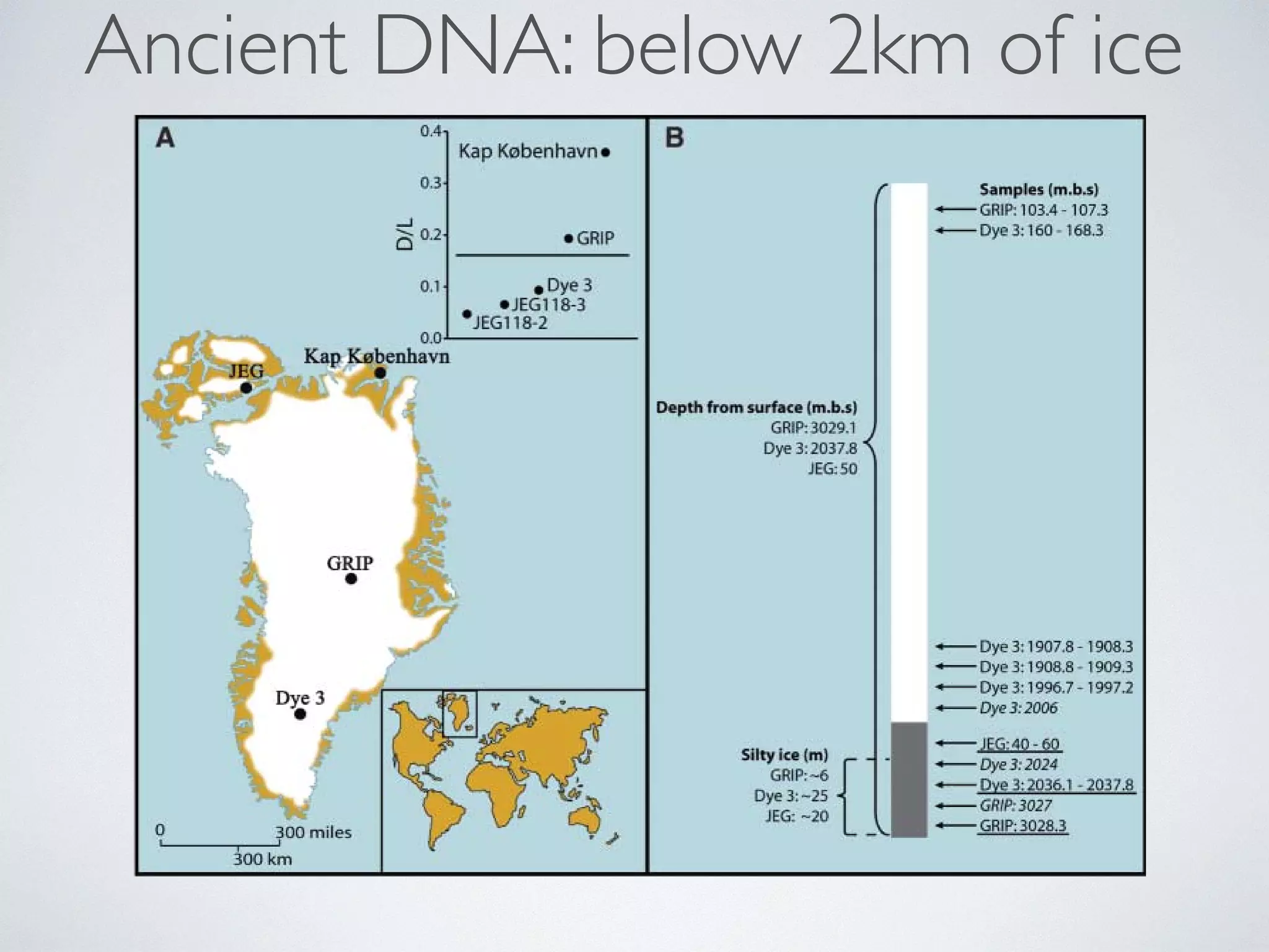
surface (m.b.s.)] indicating the depth of the cores and the positions of the Dye 3, GRIP, and JEG
samples analyzed for DNA, DNA/amino acid racemization/luminescence (underlined), and 10Be/36Cl
(italic). The control GRIP samples are not shown. The lengths (in meters) of the silty sections are
also shown.
Table 1. Plant and insect taxa obtained from the JEG and Dye 3 silty ice
samples. For each taxon (assigned to order, family, or genus level), the
genetic markers (rbcL, trnL, or COI), the number of clone sequences
supporting the identification, and the probability support (in percentage)
are shown. Sequences have been deposited in GenBank under accession
numbers EF588917 to EF588969, except for seven sequences less than 50
bp in size that are shown below. Their taxon identifications are indicated
by symbols.
Order Marker Clones Support (%) Family Marker Clones Support (%) Genus Marker Clones Support (%)
JEG sample
Rosales rbcL 3 90–99
Malpighiales rbcL
trnL
2
5
99–100
99–100
Salicaceae rbcL
trnL
2
4
99–100
100
Saxifragales rbcL 3 92–94 Saxifragaceae rbcL 2 92 Saxifraga rbcL 2 91
Dye 3 sample
Coniferales rbcL
trnL
44
27
97–100
100
Pinaceae* rbcL
Spruce
Pine
It is difficult to obtain fossil data from the 10% of Earth’s terrestrial surface that is covered by thick
glaciers and ice sheets, and hence, trnL
knowledge of the paleoenvironments of these regions has
remained limited. We show that DNA and amino acids from buried organisms can be recovered
from the basal sections of deep ice cores, enabling reconstructions of past flora and fauna. We
show that high-altitude southern Greenland, currently lying below more than 2 kilometers of ice,
was inhabited by a diverse array of conifer trees and insects within the past million years. The
results provide direct evidence in support of a forested southern Greenland and suggest that many
deep ice cores may contain genetic records of paleoenvironments in their basal sections.
The environmental histories of high-latitude
20
25
100
100
Picea
Pinus†
rbcL
trnL
20
17
99–100
90–99
Taxaceae‡ rbcL
trnL
23
2
91–98
100
Poales§ rbcL
trnL
67
17
99–100
97–100
Poaceae§ rbcL
Grasses
trnL
67
13
99–100
100
Asterales rbcL
trnL
18
27
90–100
100
Asteraceae rbcL
trnL
2
27
91
100
Fabales rbcL
trnL
10
3
99–100
99
Fabaceae rbcL
Legumes
trnL
10
3
99–100
99
Fagales rbcL
trnL
10
12
95–99
100
Betulaceae rbcL
regions such as Greenland and Antarctica
are poorly understood because trnL
much of
8
11
The samples studied come from the basal
93–97
98–100
Alnus rbcL
impurity-rich (silty) ice sections of the 2-km-long
trnL
7
9
91–95
98–100
Dye 3 core from south-central Greenland
Lepidoptera COI 12 the 97–fossil 99
evidence is hidden below kilometer-thick
*Env_2, trnL ATCCGGTTCATGAAGACAATGTTTCTTCTCCTAAGATAGGAAGGG. ice sheets (1–Env_3). 3, We trnL test ATCCGGTTCATGAAGACAATGTTTCTTCTCCTAATATAGGAAGGG. the idea that the
Env_4, trnL ATCCGGTTCATGAGGACAATGTTTCTTCTCCTAATA-TAGGAAGGG.
(4), the 3-km-long Greenland Ice Core Project
(GRIP) core from the summit of the Greenland
ice sheet (5), and the Late Holocene John Evans
Glacier on Ellesmere Island, Nunavut, northern
Canada (Fig. 1). The last-mentioned sample was
included as a control to test for potential exotic
DNA because the glacier has recently overridden
a land surface with a known vegetation cover
(6). As an additional test for long-distance
atmospheric dispersal of DNA, we included
†Env_5, trnL CCCTTCCTATCTTAGGAGAAGAAACATTGTCTTCATGAACCGGAT. Env_6, trnL TTTCCTATCTTAGGAGAAGAAACATTGTCTTCATGAACCGGAT. ‡Env_1, trnL ATCCGTATTATAG-GAACAATAATTTTATTTTCTAGAAAAGG.
basal sections of deep ice cores can act as
archives for ancient biomolecules.
§Env_7, trnL CTTTTCCTTTGTATTCTAGTTCGAGAATCCCTTCTCAAAACACGGAT.
112 6 JULY 2007 VOL 317 SCIENCE www.sciencemag.org
of the frozen control for potential have entered the cracks or during Polymerase chain the plasmid DNA of the outer interior, confirming had not penetrated Using PCR, we short amplicons the chloroplast DNA trnL intron from from the Dye 3 and samples. From Dye amplicons of invertebrate subunit I (COI) mitochondrial Attempts to reproducibly the GRIP silty ice Formation sediments results are consistent data demonstrating of biomolecules Evans Glacier silty because these samples younger (John Evans sample (Fig. 1A, DNA from the five and Pleistocene samples from the (volumes: 100 g the samples studied of vertebrate mtDNA.
1Centre for Ancient Genetics, University of Copenhagen,
A previous study of short sequences by means Search Tool likely (15). Denmark. 2BioArch, Departments of Biology and Archaeology,
University of York, UK. 3Bioinformatics Centre, University of
Copenhagen, Denmark. 4Centre for Comparative Genomics,
University of Copenhagen, Denmark. 5Max Planck Institute for
Evolutionary Anthropology, Germany. 6Murdoch University
Ancient DNA Research Laboratory, Murdoch University,
Willerslev 2007
Birch
Butterflies
Daisies/Sunflower](https://image.slidesharecdn.com/sbc174evolution2014-week3-141006054822-conversion-gate01/75/Sbc174-evolution2014-week3-97-2048.jpg)

![Independent
colonization events
less than 10,000
The freshwater populations, despite their younger age, are divergent both from the oceanic ancestral populations and each other, consistent with our supposition that they represent
independent colonizations from the ancestral oceanic population.
These results are remarkably similar to results obtained previously
from some of these same populations using a small number microsatellite and mtDNA markers [55]. This combination large amounts of genetic variation and overall low-to-moderate
differentiation between populations, phenotypic evolution years in the ago
coupled with recent and freshwater populations, presents ideal situation for identifying genomic regions that have responded
to various kinds of natural selection.
Patterns of genetic diversity distributed across the
genome
To assess genome-wide patterns we examined mean nucleotide
diversity in Saltwater:
(p) and heterozygosity (H) using a Gaussian smoothing function across each linkage group (Figure 4 and S1). Although the overall mean diversity and heterozygosity are 0.00336 and 0.00187, respectively, values vary widely the genome. Nucleotide diversity within genomic regions from 0.0003 to over 0.01, whereas heterozygosity values from 0.0001 to 0.0083. This variation in diversity across genome provides important clues to the evolutionary processes
that in are Freshwater:
maintaining genetic diversity. For example, expected (p) and observed (H) heterozygosity largely correspond,
they differ at a few genomic regions (e.g., on Linkage Group Genomic regions that exhibit significantly (p,1025) low levels diversity and heterozygosity (e.g. on LG II and V, Figure and Figure S1) may be the result of low mutation low recombination rate, purifying or positive selection consistent across populations, or some combination of [9,36,105–107].
F
F
F
S
S
F = Freshwater
S = Saltwater
Bill Cresko et al;
Different amounts of
armor plating](https://image.slidesharecdn.com/sbc174evolution2014-week3-141006054822-conversion-gate01/75/Sbc174-evolution2014-week3-102-2048.jpg)
![RAD = Restriction-site Associated DNA sequencing
each locus sequenced
5–10 times per fish.
F
F
F = Freshwater
Bill Cresko et al;
The freshwater populations, despite their younger age, are more
divergent both from the oceanic ancestral populations and from
each other, consistent with our supposition that they represent
independent colonizations from the ancestral oceanic population.
These results are remarkably similar to results obtained previously
from some of these same populations using a small number of
microsatellite and mtDNA markers [55]. This combination of
large amounts of genetic variation and overall low-to-moderate
differentiation between populations, coupled with recent and rapid
phenotypic evolution in the freshwater populations, presents an
ideal situation for identifying genomic regions that have responded
to various kinds of natural selection.
Patterns of genetic diversity distributed across the
genome
To assess genome-wide patterns we examined mean nucleotide
diversity (p) and heterozygosity (H) using a Gaussian kernel
smoothing function across each linkage group (Figure 4 and Figure
S1). Although the overall mean diversity and heterozygosity values
are 0.00336 and 0.00187, respectively, values vary widely across
the genome. Nucleotide diversity within genomic regions ranges
from 0.0003 to over 0.01, whereas heterozygosity values range
from 0.0001 to 0.0083. This variation in diversity across the
genome provides important clues to the evolutionary processes
that are maintaining genetic diversity. For example, while
expected (p) and observed (H) heterozygosity largely correspond,
they differ at a few genomic regions (e.g., on Linkage Group XI).
Genomic regions that exhibit significantly (p,1025) low levels of
diversity and heterozygosity (e.g. on LG II and V, Figure 4
and Figure S1) may be the result of low mutation rate,
low recombination rate, purifying or positive selection that is
consistent across populations, or some combination of factors
[9,36,105–107].
In contrast, other genomic regions, such as those on LG III and
XIII (Figure 4), show very high levels of both diversity and
heterozygosity. The most striking such region, found near the end
Figure 1. Location of oceanic and freshwater populations
examined. Threespine stickleback were sampled from three freshwa-ter
(Bear Paw Lake [BP], Boot Lake [BL], Mud Lake [ML]) and two oceanic
Population Genomics in Stickleback
F
S
S
S = Saltwater
20 fish per population
45,789 loci genotyped](https://image.slidesharecdn.com/sbc174evolution2014-week3-141006054822-conversion-gate01/75/Sbc174-evolution2014-week3-103-2048.jpg)
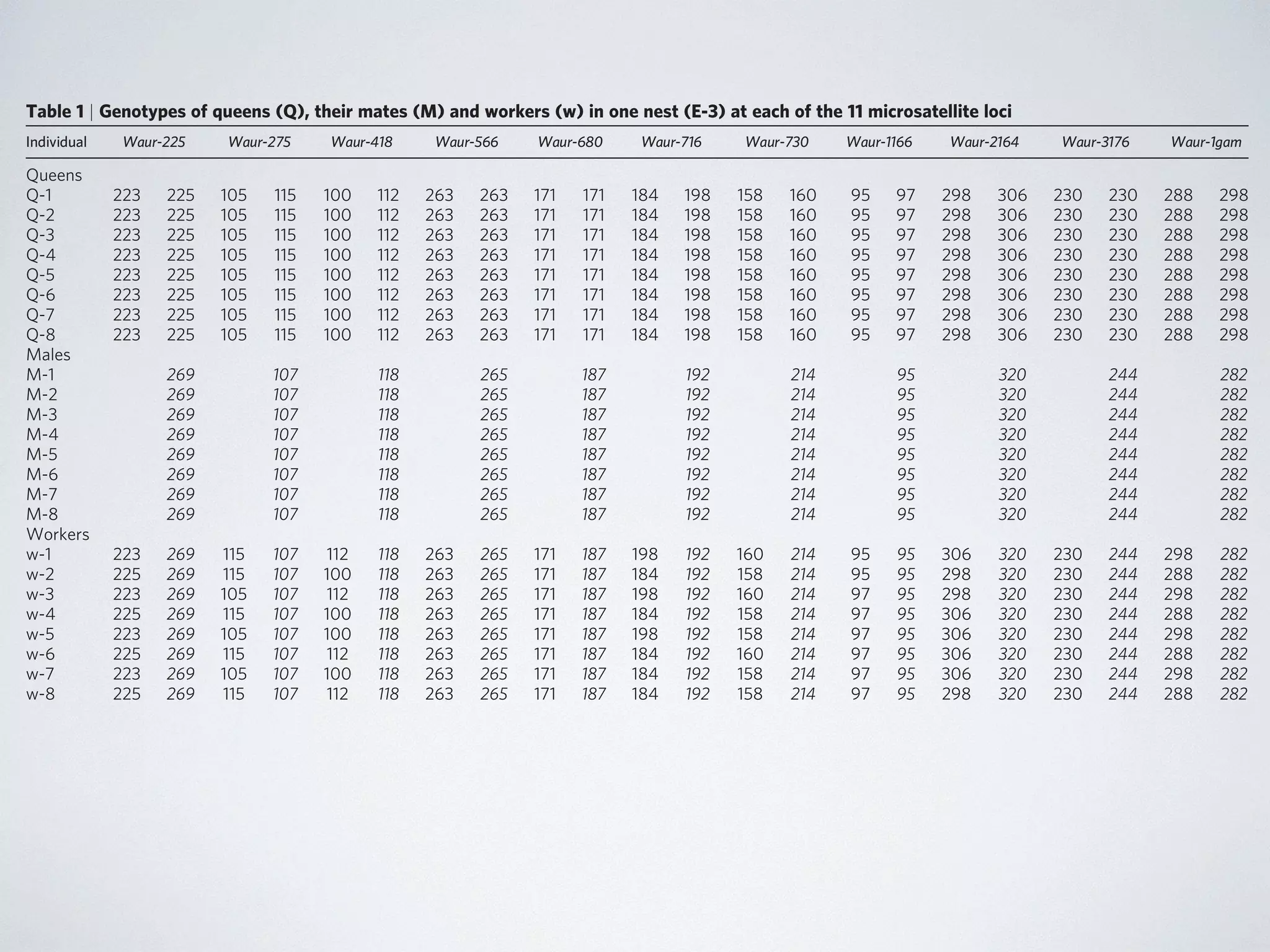
![Downloaded from rspb.royalsocietypublishing.org on January Here:
reproduction (that is, by ameiotic parthenogenesis). In 33 of the nests, all queens (n ¼ 135) and gynes (n ¼ 9) cohabiting in the same
nest shared an identical genotype at each of the 11 loci (Table 1 Fig. 1). The single exception was nest B-12, in which queens differed
at 1 of the 11 loci: four queens were heterozygous at Waur-2164
and the remaining three queens were homozygous for one of two alleles. This variation probably reflects a mutation or recombi-nation
* workers carry DNA
from mother & father
* new queens are 100%
clones of their mother
* new males are 100%
clones of their father
event in one queen followed by clonal reproduction within
the nest. The history of this genetic change could be reconstructed
from the genotypes of queens collected in neighbouring nests (Figs and 2). Nine queens from two neighbouring nests (B-11 and B-had the same genotype as the four heterozygous queens for locus
Waur-2164, indicating that the mutation or recombination event
probably was from a heterozygote to a homozygote queen. The three
homozygote queens from nest B-12 had a unique genotype in population, which further supports this interpretation.
A comparison between nests supports the view of restricted female
gene flow, with budding being the main mode of colony formation.
Within three of the five sites of collection (A, C and D) all queens the same genotype at the 11 loci (Fig. 2). In one of the two other 2680 M. Pearcy et al. Sib mating without inbreeding
(B), all queens from 8 of the 17 nests also had an identical genotype,
whereas in the other site (E) the queen genotypes were different in three nests sampled. Taken together, these data indicate that queens
belonging to the same lineage of clonally produced individuals
frequently head closely queen located nests. mate
Moreover, genetic differen-tiation
between sites was very strong, with a single occurrence genotypes shared between sites (the eight queens of nest E-3 genotypes identical to the most common genotype found at site showing that gene flow by females is extremely restricted.
In stark contrast to reproductive females, the genotypic analyses
revealed that workers are produced by normal sexual reproduction
(Table 1). Over all 31 queenright nests, each of the 248 genotyped
workers had, at seven or more loci, one allele that was absent queens of their nest. Moreover, the 232 workers from the 29 nests which the sperm in the queen’s spermathecae was successfully
obtained had all genotypes consistent with those expected under
Figure 2 | Neighbour-joining dendrogram of the genetic (allele-shared)
distances between queens (Q), gynes (G) and male sperms (M) collected
over all the five sites (A–E). The collection number of each nest is given
two other ant species: emeryi [21,22]. study, it is likely also translates sib mating on the W. auropunctata studies have shown derive from a characterized by single male genotype. and a single male is also compatible a single mated gynes workers males
Interestingly, lay male eggs that least two potential being clonally genome could [21]. Indeed, Figure 2. Clonal reproduction in queens and males. The
figure summarizes the reproduction system of P. longicornis
in the study population. Maternal (light) and paternal
(dark) chromosomes are displayed. Contribution to the
genome of the offspring is indicated by arrows (dashed](https://image.slidesharecdn.com/sbc174evolution2014-week3-141006054822-conversion-gate01/75/Sbc174-evolution2014-week3-108-2048.jpg)
![Example 3: Species-interactions via
DNA sequencing
Correspondences Screening mammal
biodiversity using
DNA from leeches
Ida Bærholm Schnell1,2,†,
Philip Francis Thomsen2,†,
Nicholas Wilkinson3,
Morten Rasmussen2,
Lars R.D. Jensen1, Eske Willerslev2,
Mads F. Bertelsen1,
and M. Thomas P. Gilbert2,*
With nearly one quarter of mammalian
species threatened, an accurate
description of their distribution and
conservation status is needed [1].
For rare, shy or cryptic species,
in the medical leech (Hirudo medicinalis)
viruses remain detectable in the blood
meal for up to 27 weeks, indicating viral
nucleic acid survival [4,5]. To examine
whether PCR amplifiable mammalian
DNA persists in ingested blood, we
fed 26 medical leeches (Hirudo spp.)
freshly drawn goat (Capra hircus)
blood (Supplemental information) then
sequentially killed them over 141 days.
Following extraction of total DNA, a
goat-specific quantitative PCR assay
demonstrated mitochondrial DNA
(mtDNA) survival in all leeches, thus
persistence of goat DNA, for at least
4 months (Figure 1A; Supplemental
information).
We subsequently applied the
method to monitor terrestrial
mammal biodiversity in a challenging
environment. Haemadipsa spp. leeches
were collected in a densely forested
biotope in the Central Annamite region
how
new
into
John
expression in
differentiation.
sex
586.
genes
central
fish.
determination
Magazine
R263
Figure 1. Monitoring mammals with leeches.
(A) Survival of mtDNA in goat blood ingested by Hirudo medicinalis over time, relative to freshly
drawn sample (100%, ca. 2.4E+09 mtDNA copies/gram blood). Mitochondrial DNA remained
detectable in all fed leeches, with a minimum observed level at 1.6E+04 mtDNA/gram blood
ingested. The line shows a simple exponential decay model, p < 0.001, R2 = 0.43 (Supplemental
information). (B) Vietnamese field site location and examples of mammals identified in Hae-madipsa
spp. leeches. From left to right: Annamite striped rabbit, small-toothed ferret-badger,](https://image.slidesharecdn.com/sbc174evolution2014-week3-141006054822-conversion-gate01/75/Sbc174-evolution2014-week3-109-2048.jpg)


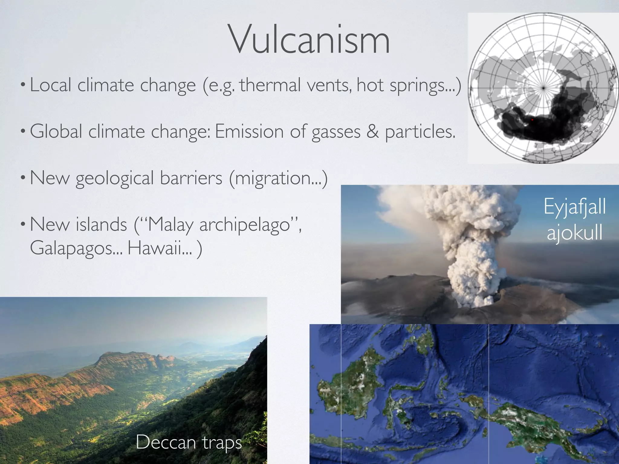
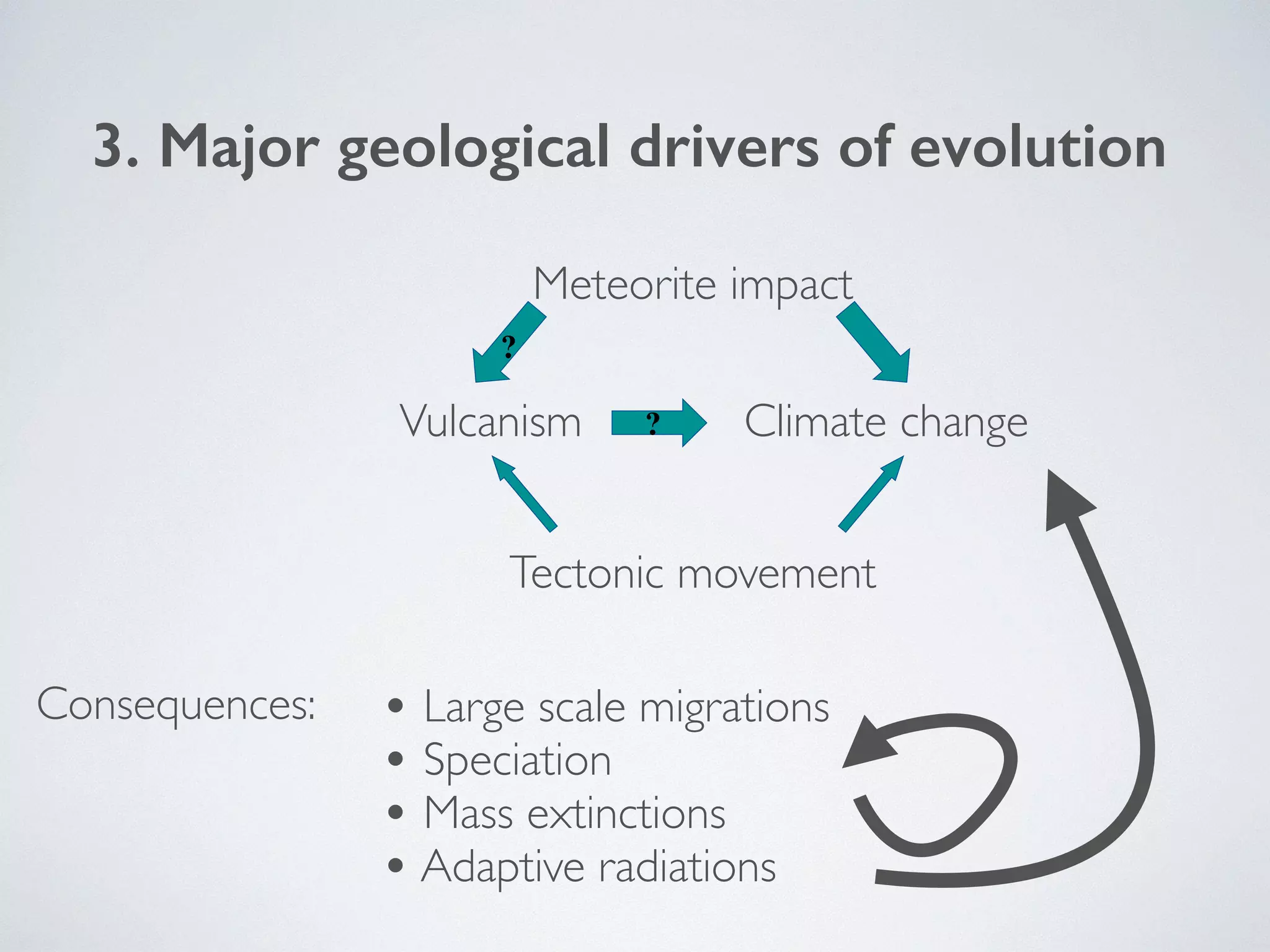
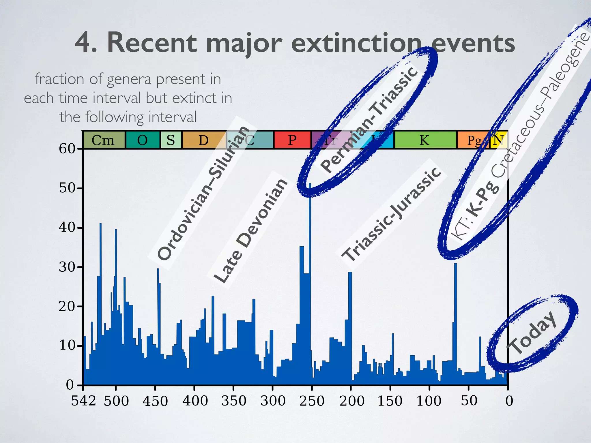
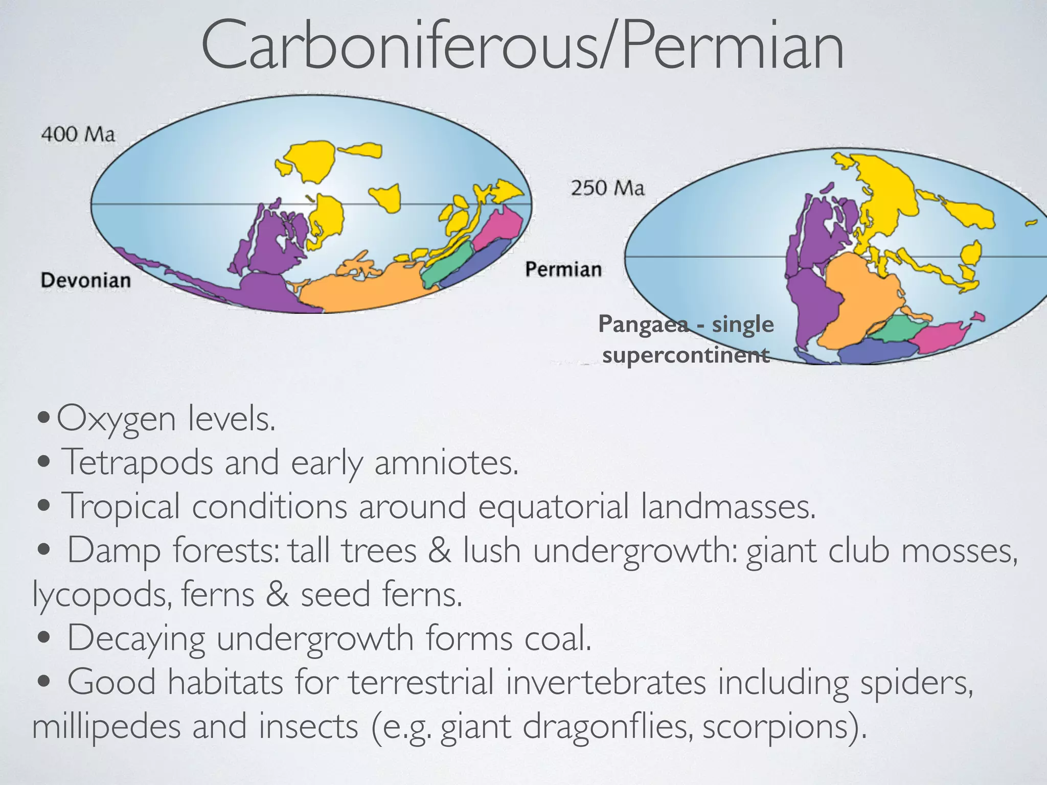
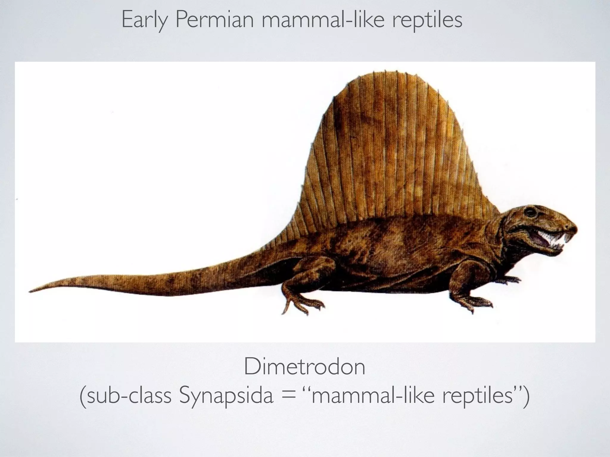
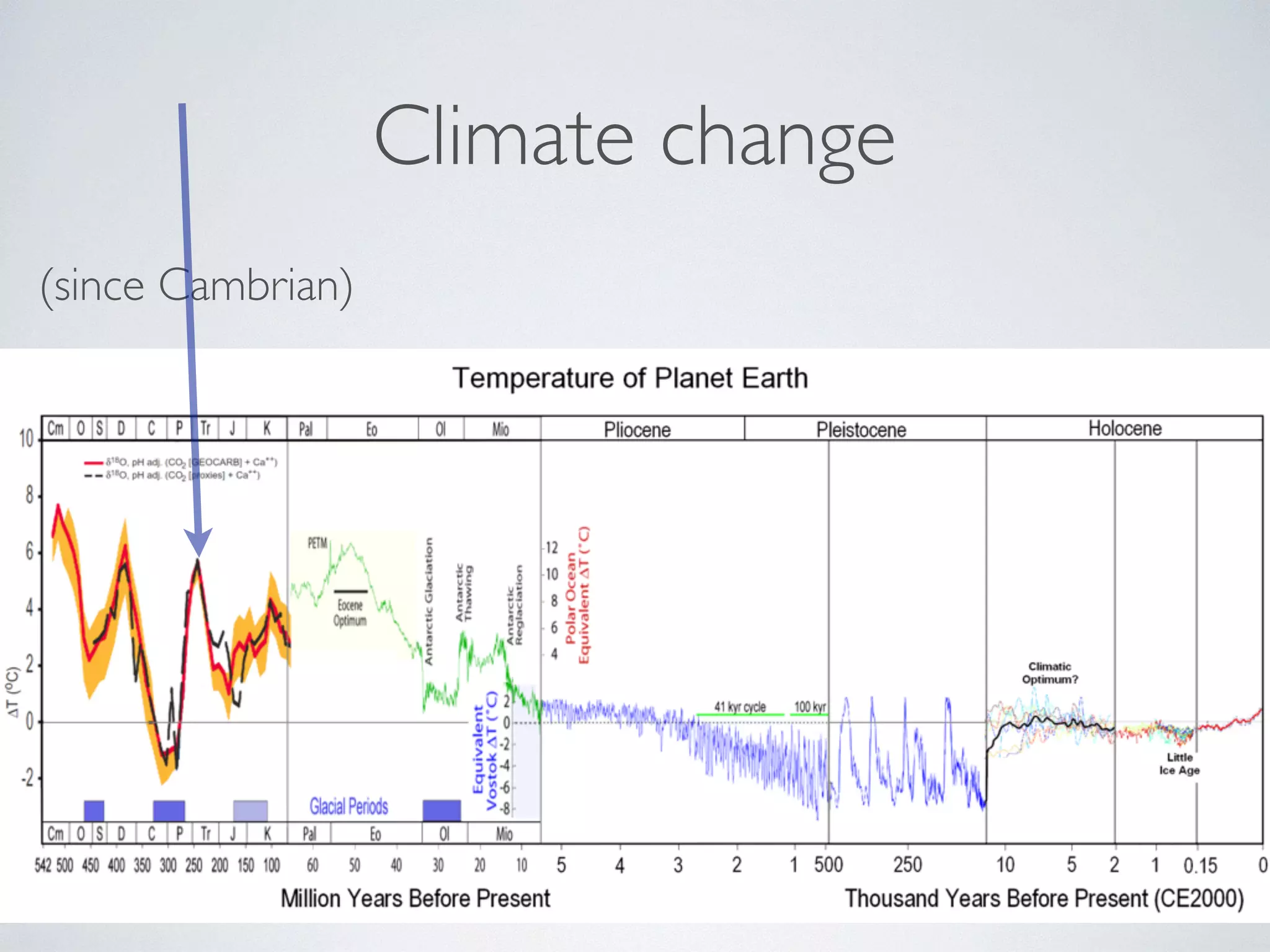
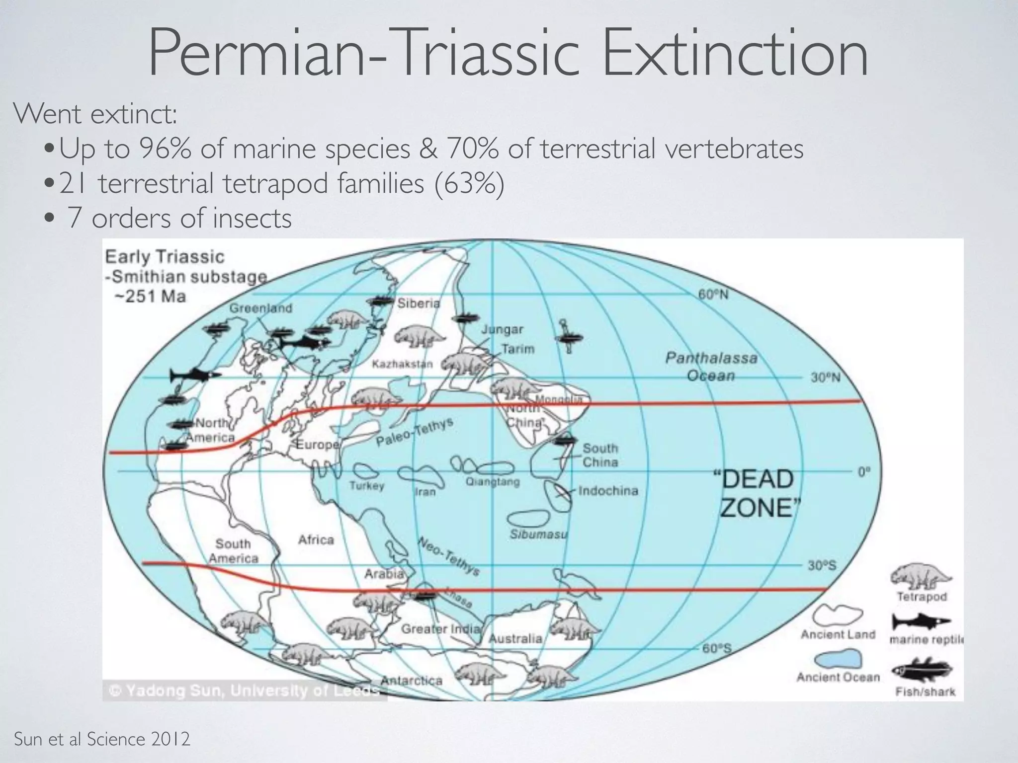
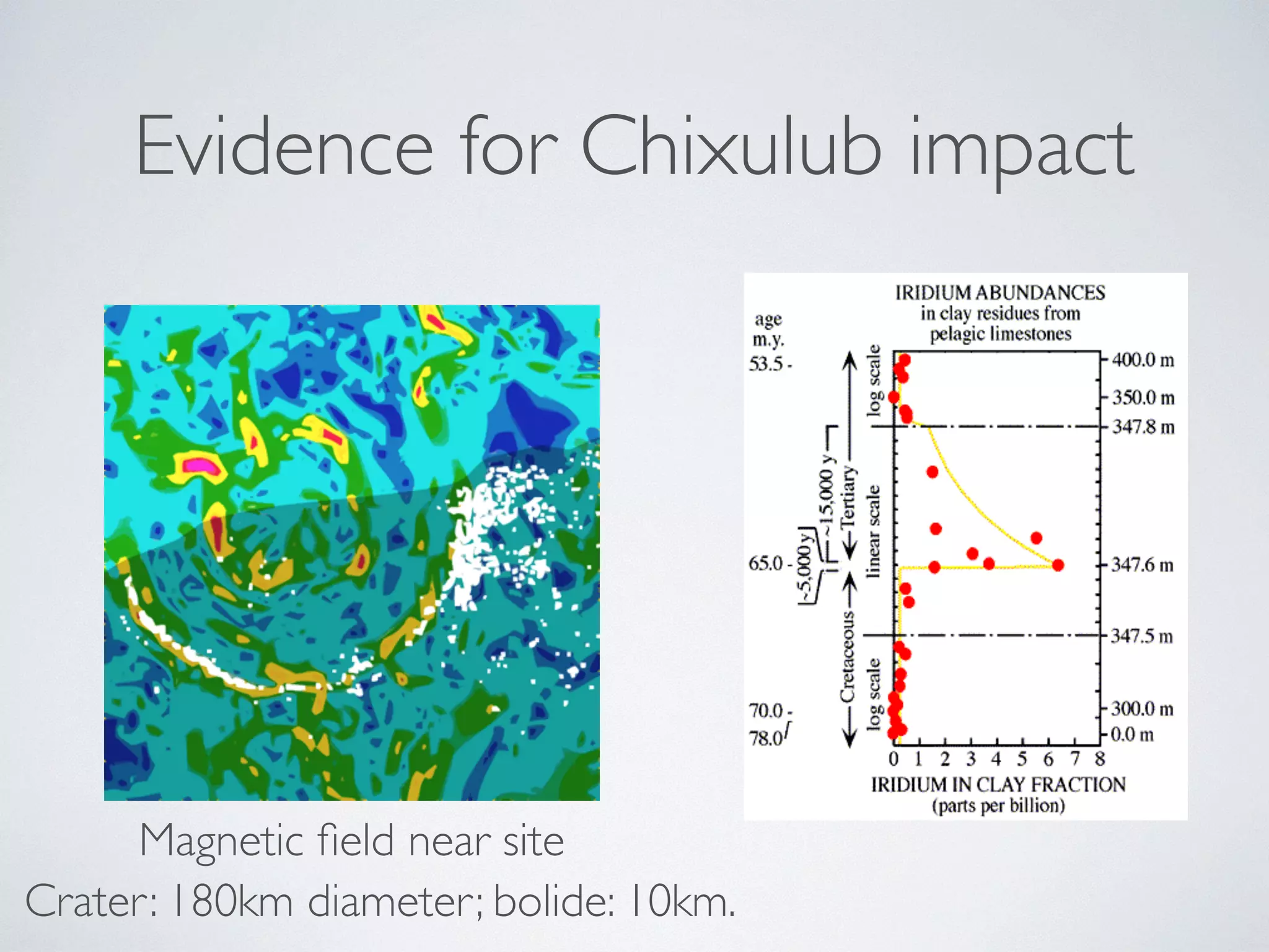
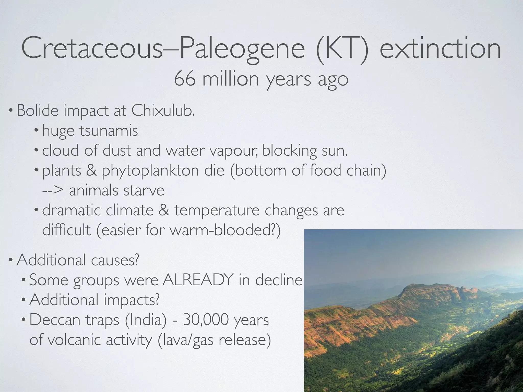
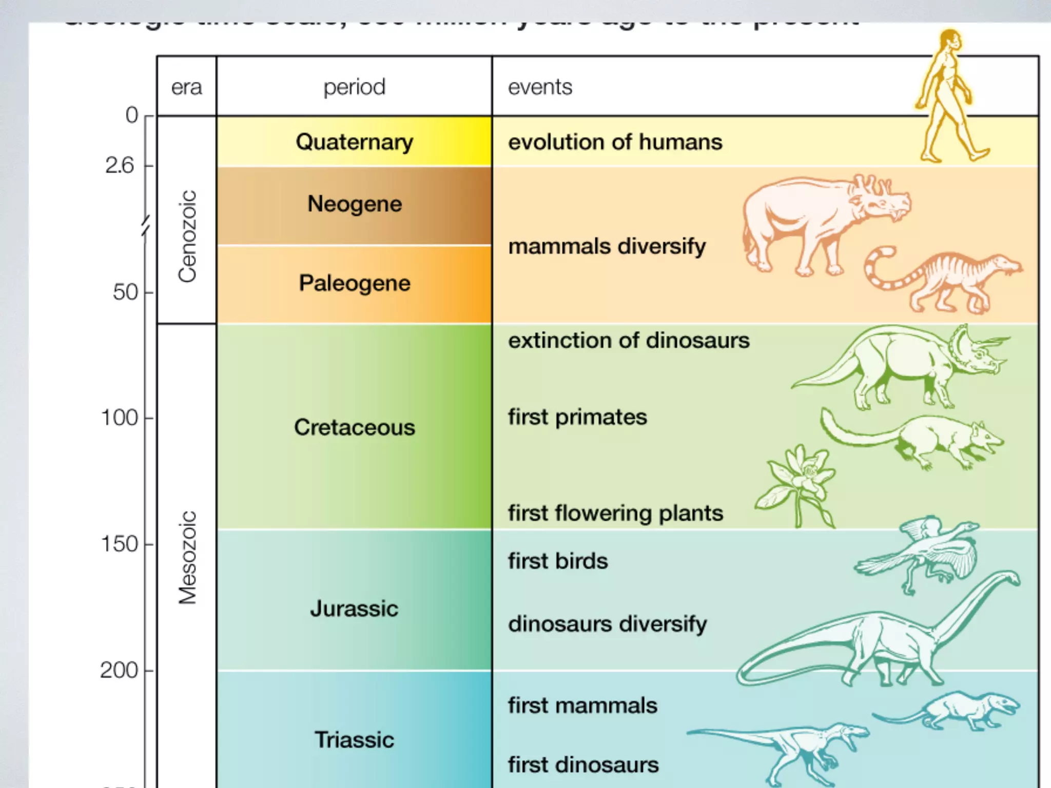
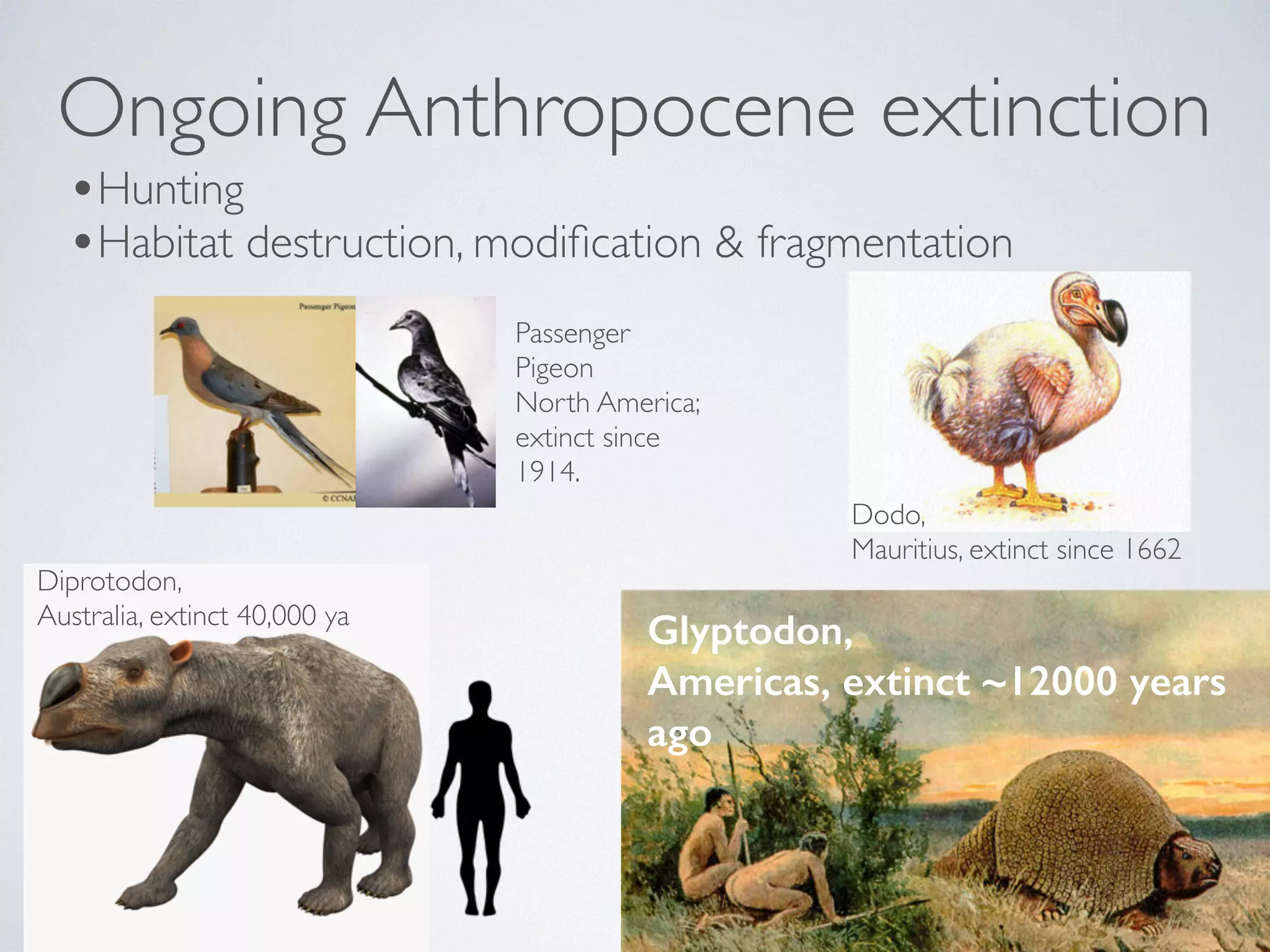
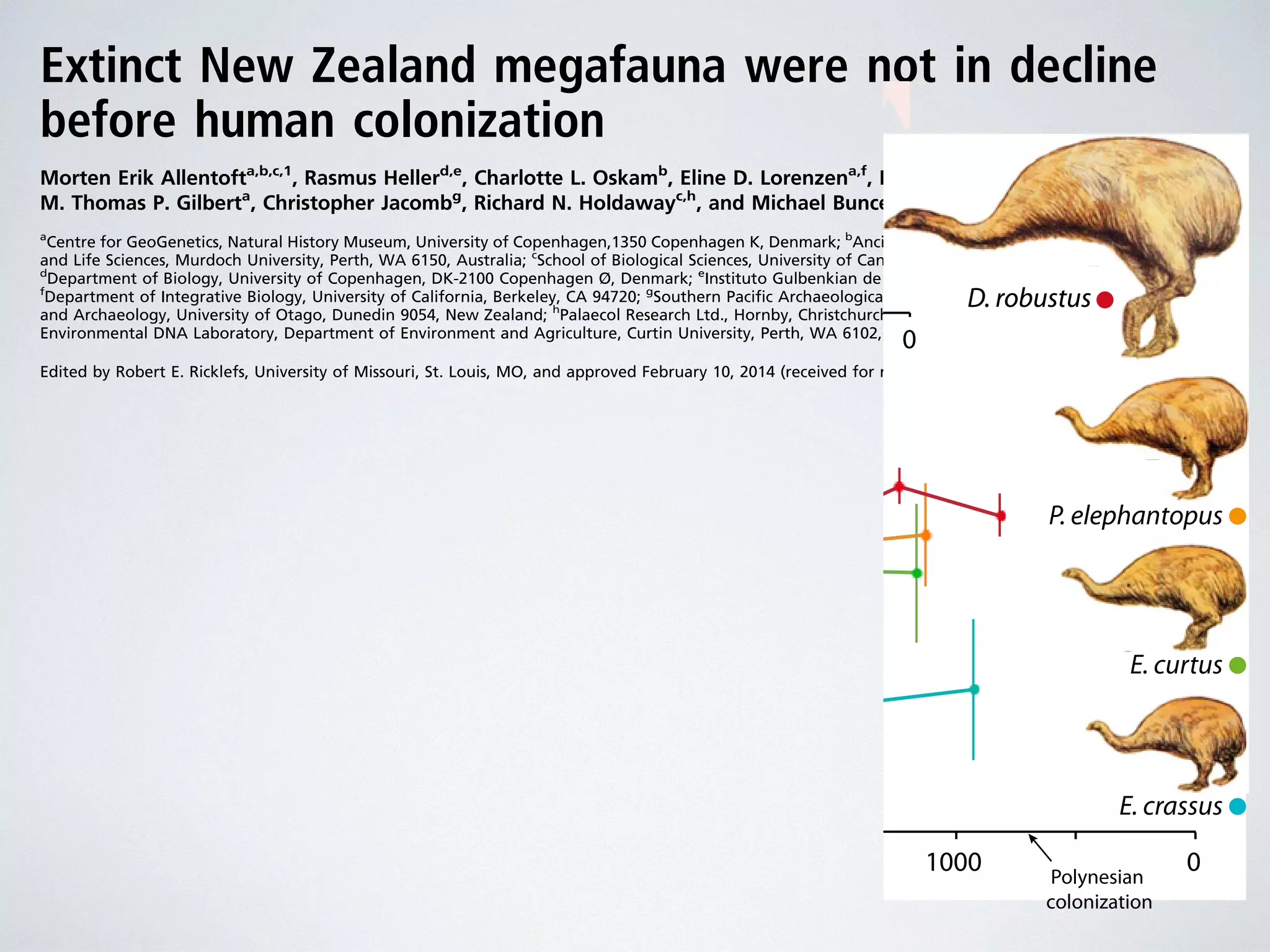
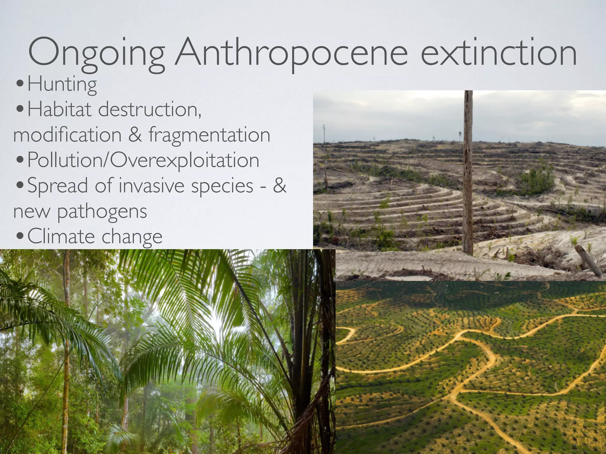
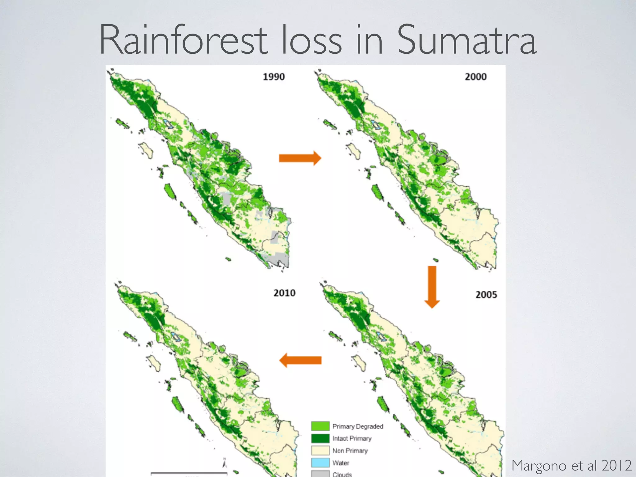
The document discusses major geological drivers of evolution on Earth over time, including tectonic movement, volcanism, climate change, and meteorite impacts. These geological forces have caused large-scale migrations, speciation events, mass extinctions, and adaptive radiations in species. Specific examples of major extinction events are described, such as the Permian-Triassic, Cretaceous-Paleogene, and more recent extinctions following human arrival and activities on various continents and islands.