Downloaded 206 times
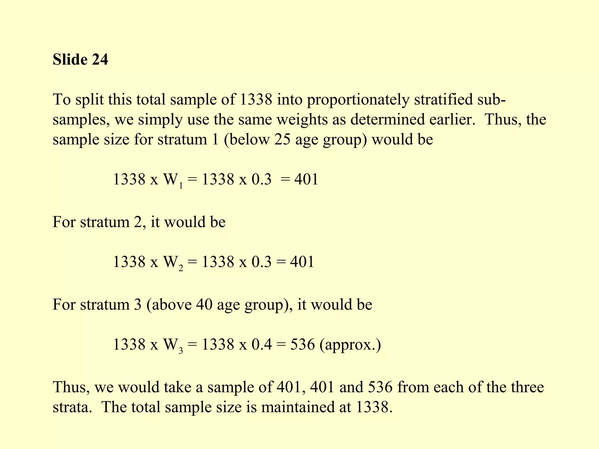
![Slide 23
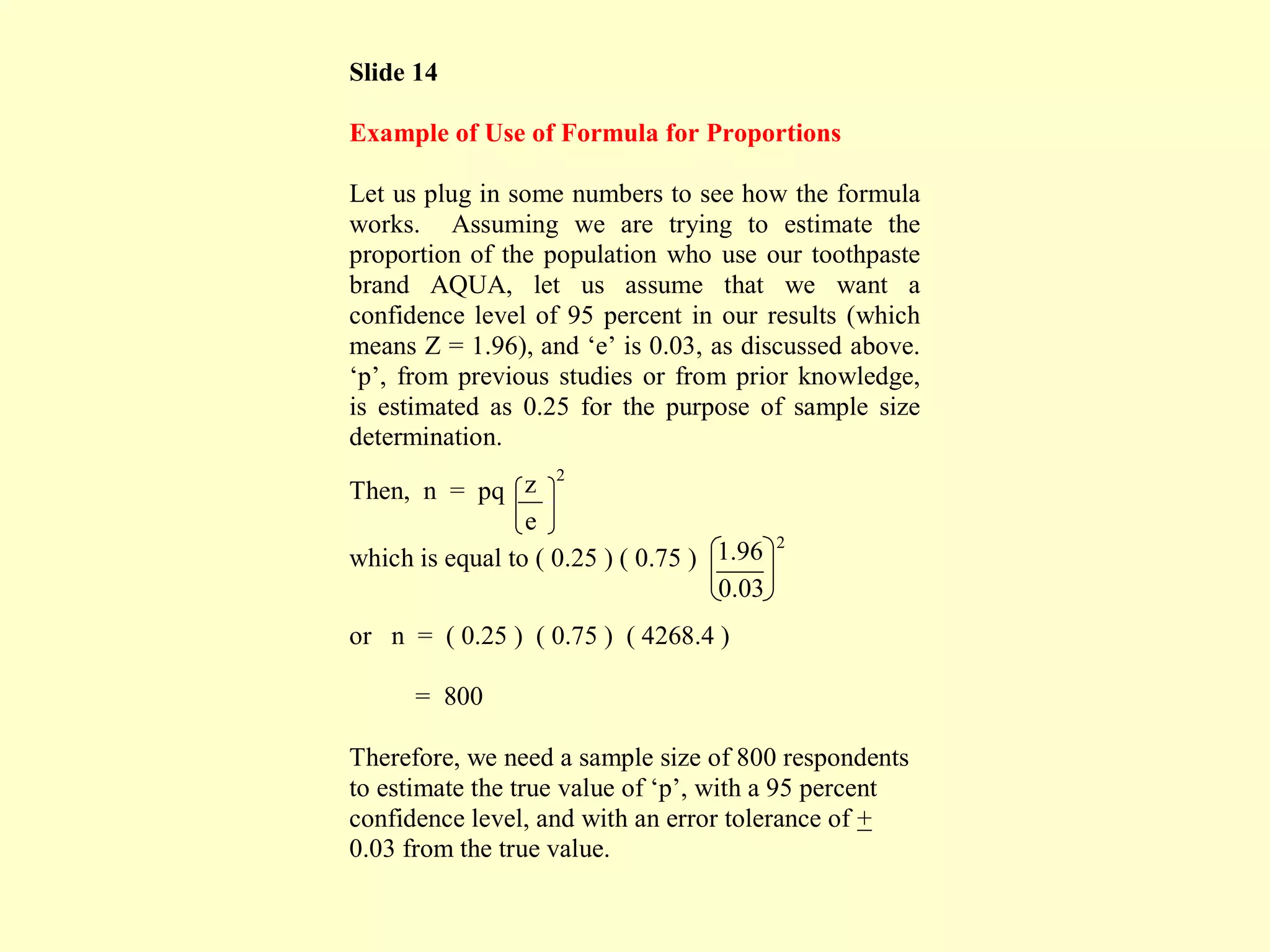
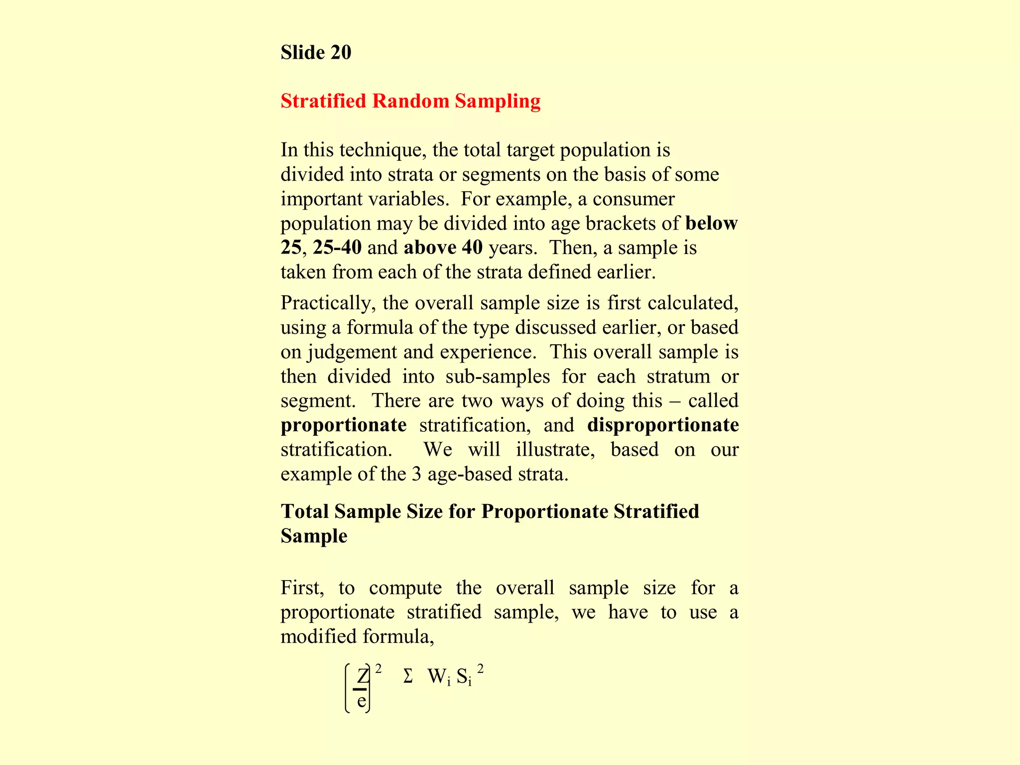
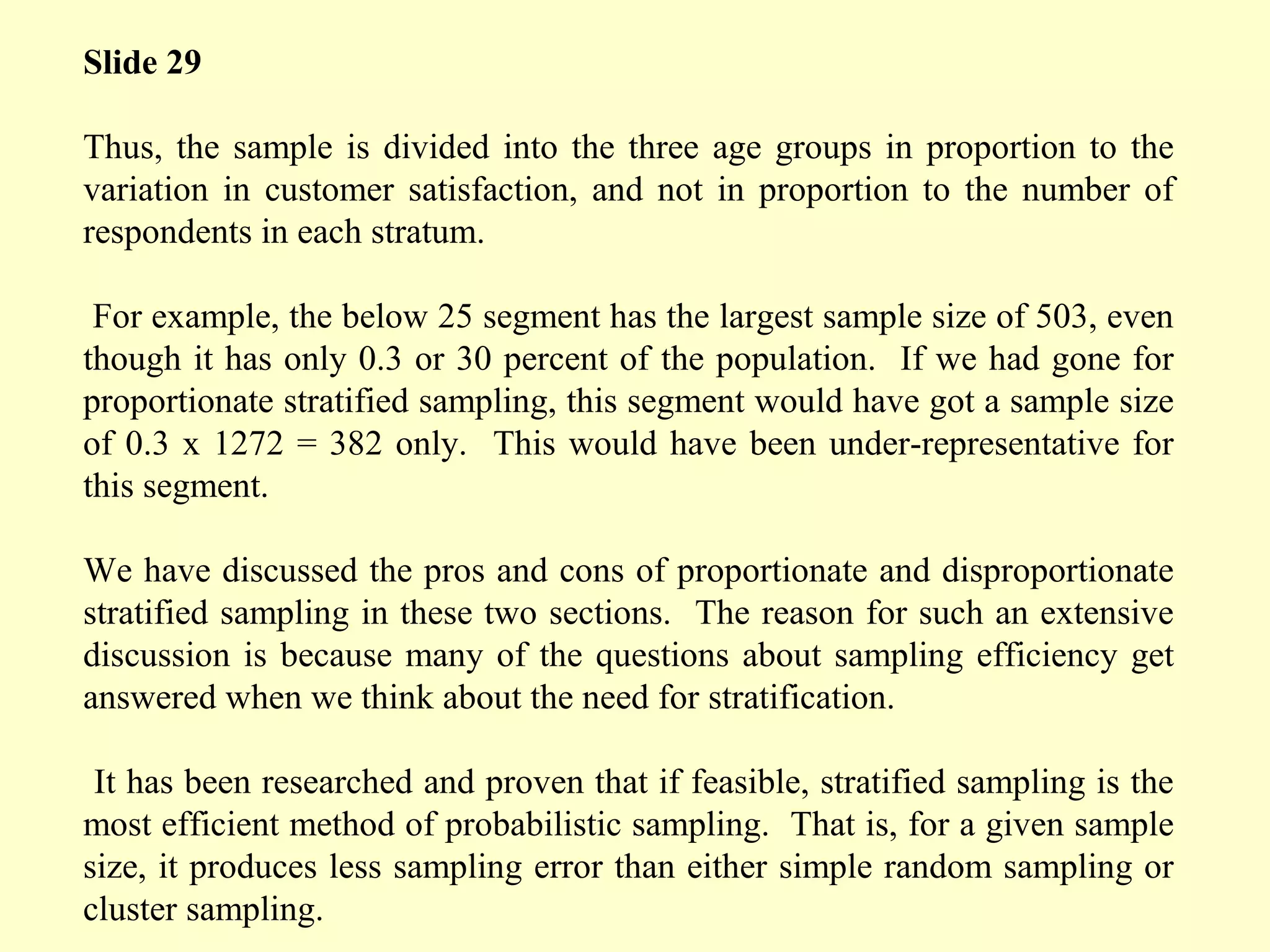
Now, applying the formula,
Z 2
n = ---- Σ Wi Si
2
, we get
e
n = 1.96 2
[ (0.3) (1.2) 2
+ (0.3) (0.9) 2
+ (0.4) (0.7) 2
]
0.05
= 1536 [0.871] = 1338 (approx.)
This is the total sample size required. (Note that if
we had used the formula for simple random sampling
discussed earlier, sample size n would have been
(using s=1 as estimated above) equal to 1536. So,
stratified sampling has led to a smaller sample size of
1338 for the same z and e values.)](https://image.slidesharecdn.com/sampling-20methods-20theory-20and-20practice-140425122404-phpapp02/75/Sampling-methods-theory-and-practice-29-2048.jpg)
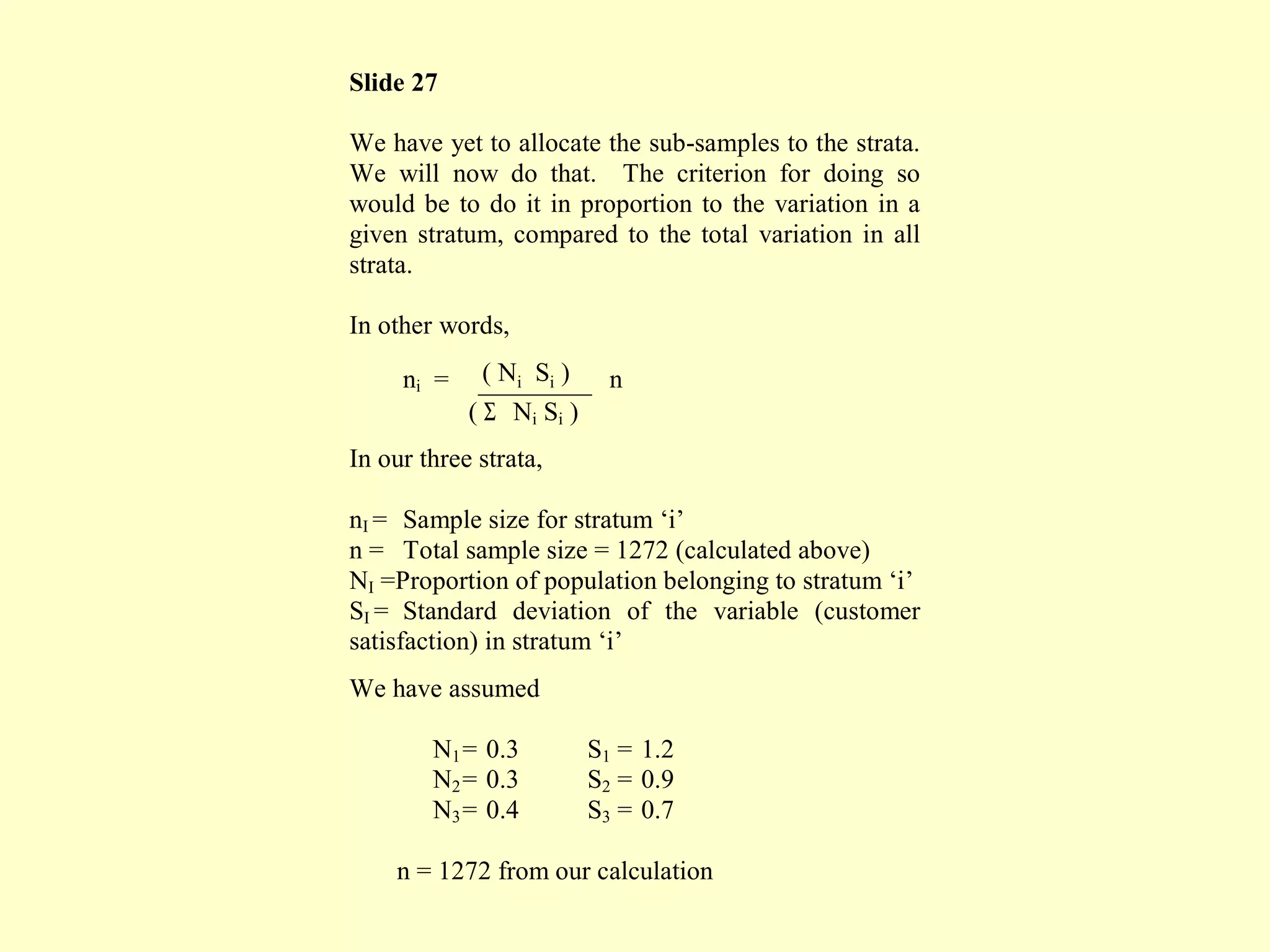
![Slide 26
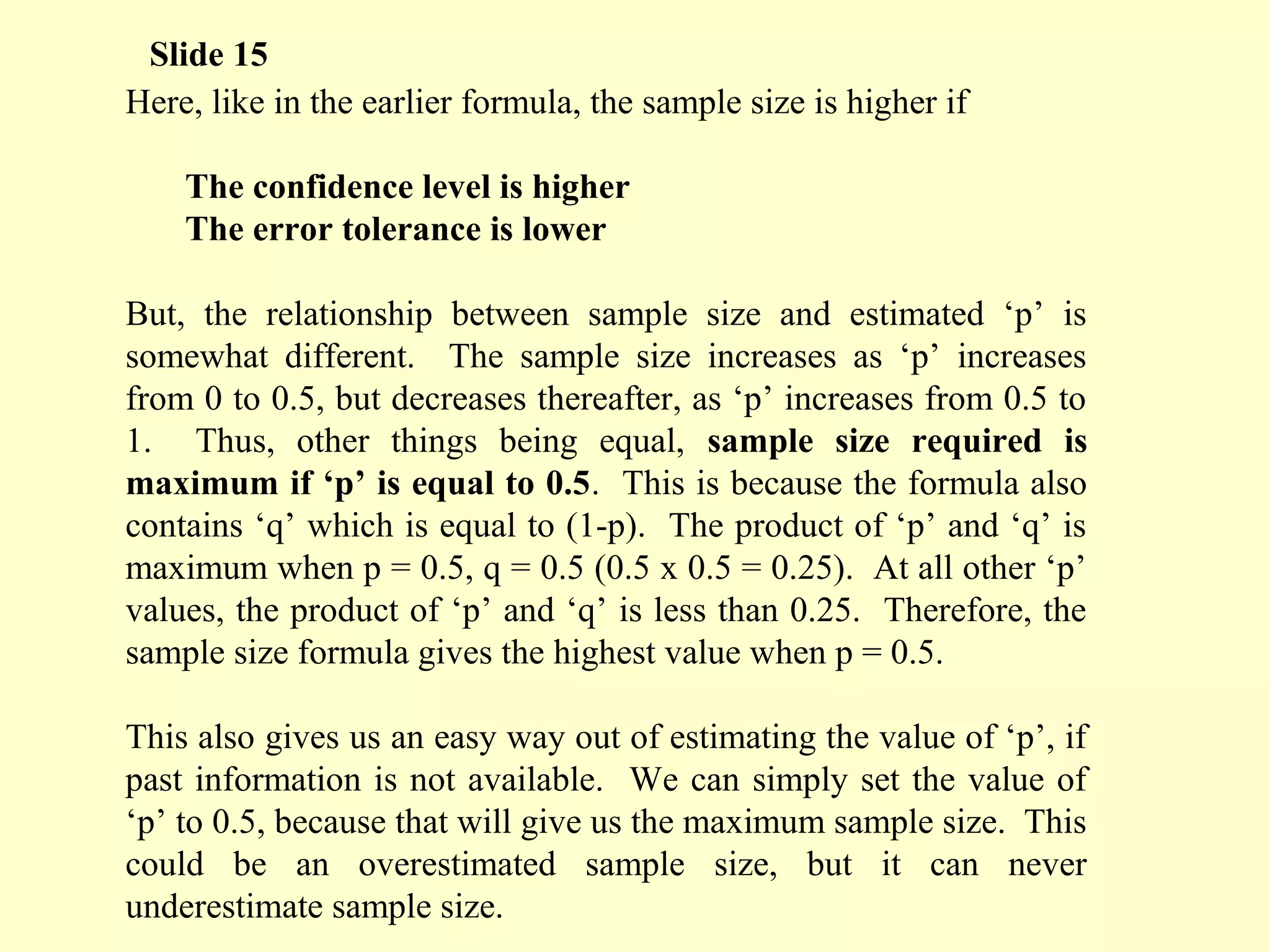
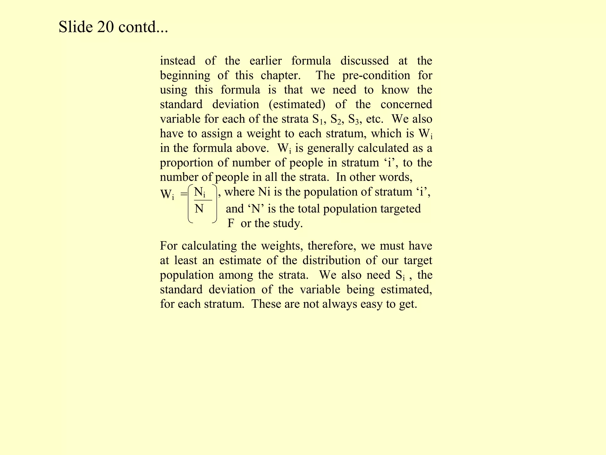
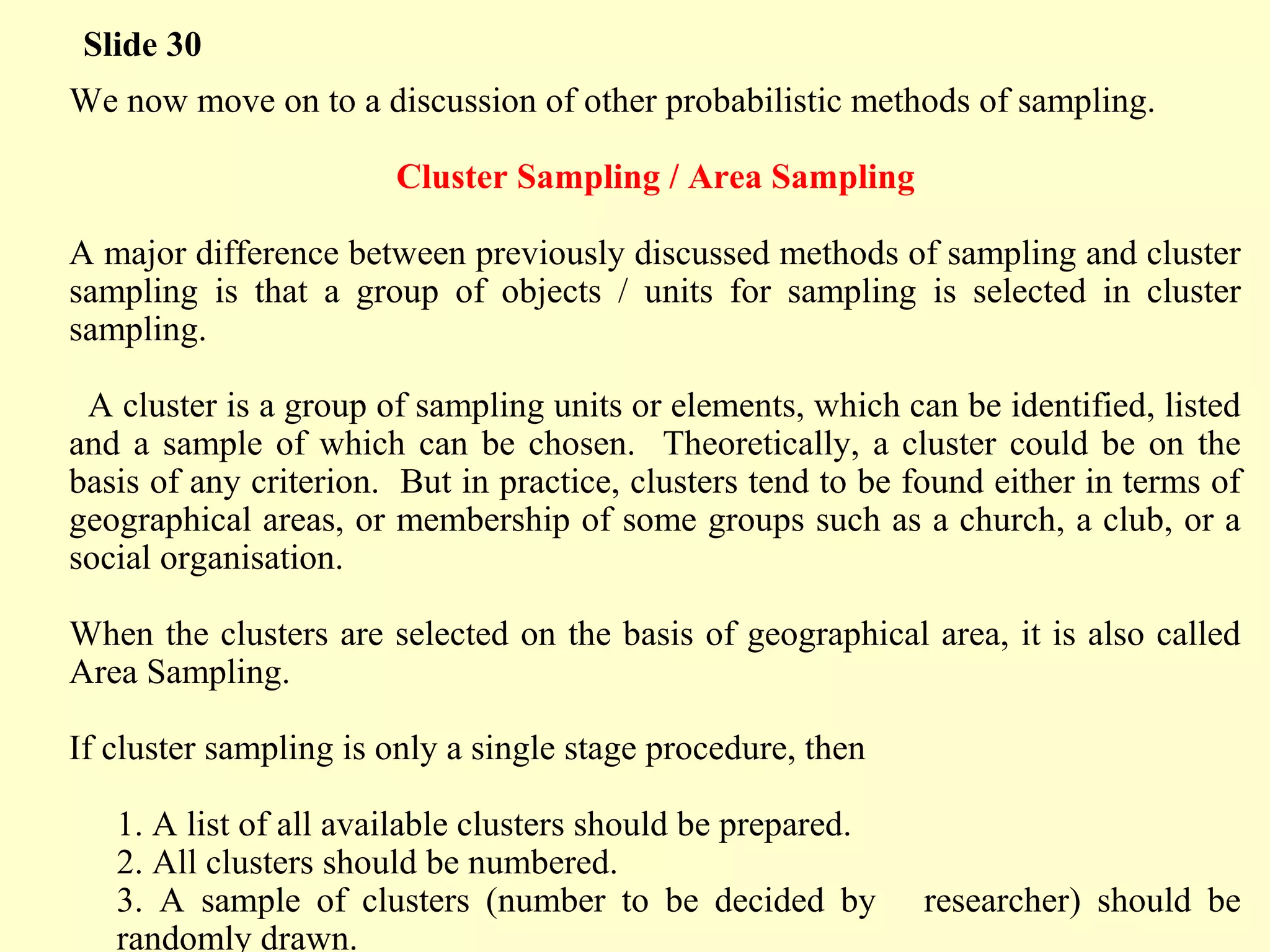
The formula for the total sample size calculation is
(for disproportionate sampling)
Z 2
n = ---- ( Σ Wi Si ) 2
e
This is slightly different from the formula used in
case of proportionate stratified sampling.
To illustrate, let us use the same example of three
age-based strata, and check how to use a
disproportionate sample in the same.
Z 2
n = ---- ( Σ Wi Si ) 2
e
n = 1.96 2
[ (0.3) (1.2) + (0.3) (0.9) + (0.4) (0.7)] 2
0.05
= (1536) (0.8281) = 1272 (approx.)
Thus, we see that compared to the proportionate
stratified sample, we have got a lower sample size,
for the same level of tolerable error (e) and Z (1.96,
95 percent confidence level). In general, we will note
that disproportionate stratified samples tend to be
more efficient (lower sample sizes are obtained), than
proportionate stratified samples, because we allocate
sample size according to the variability in the strata.](https://image.slidesharecdn.com/sampling-20methods-20theory-20and-20practice-140425122404-phpapp02/75/Sampling-methods-theory-and-practice-32-2048.jpg)

The document discusses key concepts related to sampling methods in marketing research. It defines sampling elements, population, sampling frame, and sampling unit. It presents formulas for calculating sample size when estimating means of continuous variables and proportions. The formula for means involves variables like confidence level (Z), standard deviation (s), and tolerable error (e). The formula for proportions uses variables like confidence level (Z), estimated proportion (p), and tolerable error (e). The document provides an example of each formula and discusses limitations of the formulas related to number of centers, multiple questions, and cell size in analysis.