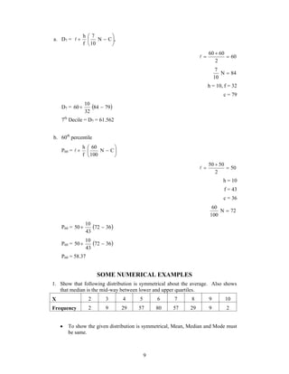
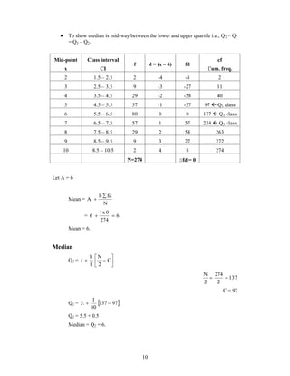
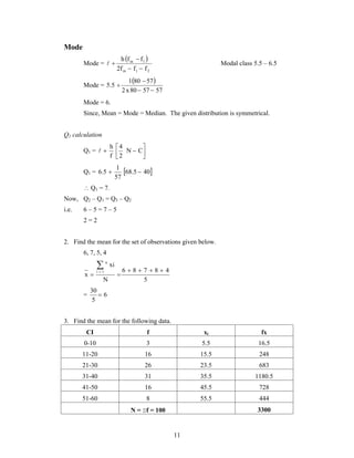
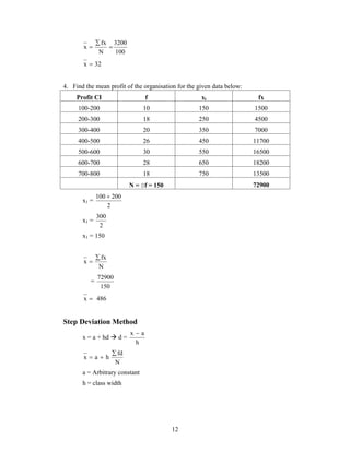
Download to read offline

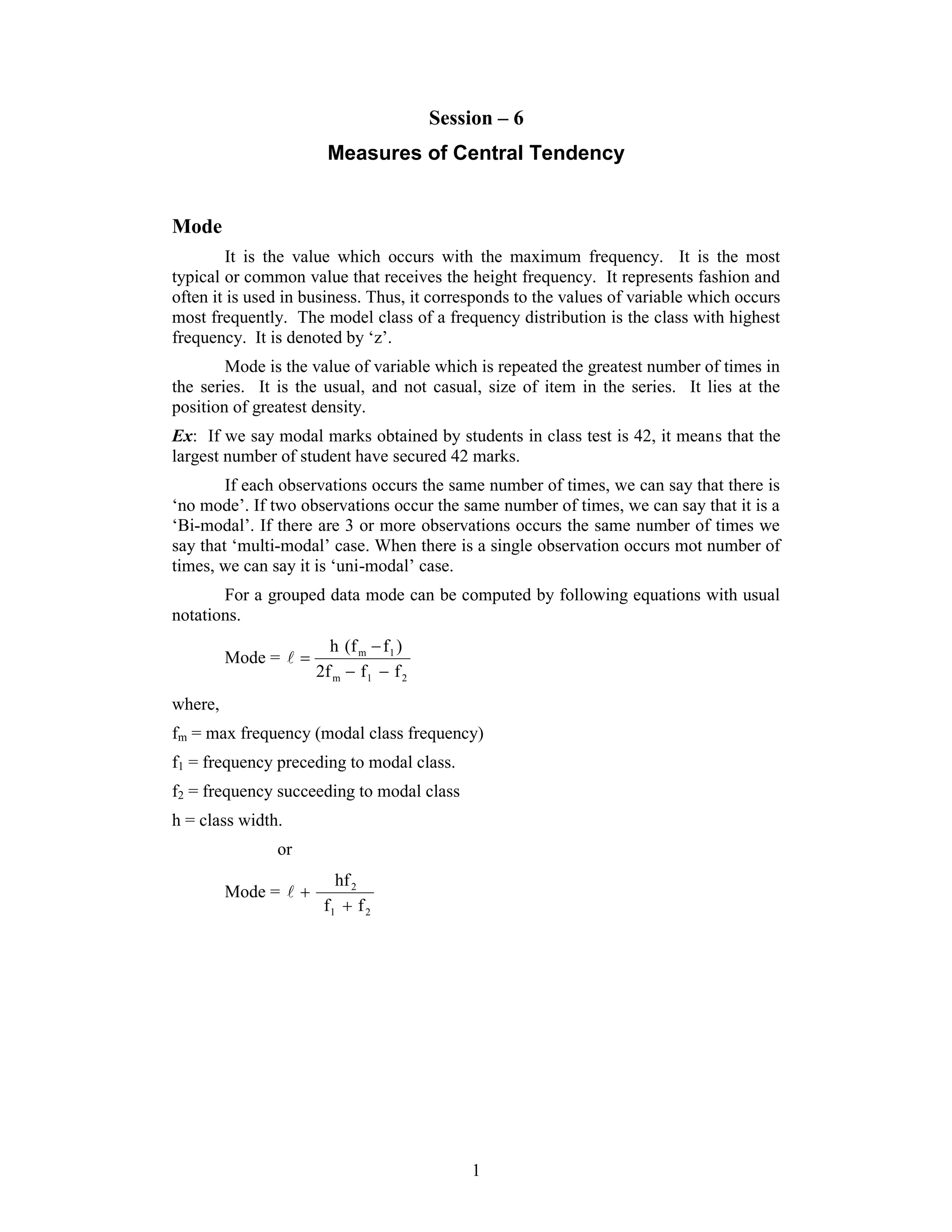
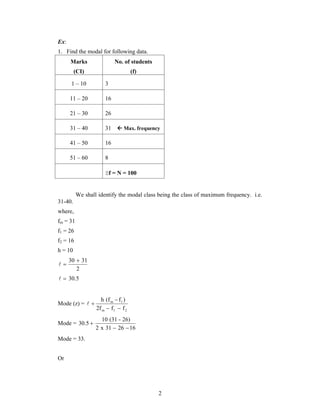
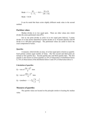


This document discusses measures of central tendency, including the mode, median, quartiles, and percentiles. It provides definitions and formulas for calculating each measure. The mode is defined as the value that occurs most frequently. The median divides the data set into two equal parts. Quartiles divide the data set into four equal parts, with the second quartile being the median. Percentiles divide the data set into 100 equal parts. Several examples are provided to demonstrate calculating the mode, median, quartiles, deciles and percentiles from data sets.