Downloaded 200 times
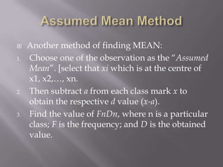
![ It‟s the „running total‟ of frequencies.
It‟s the frequency obtained by adding the of all
the preceding classes.
When the class is taken as less than [the Upper
limit of the CI], the cumulative frequencies is
said to be the less than type.
When the class is taken as more than [the lower
limit of the CI], the cumulative frequencies is
said to be the more than type.](https://image.slidesharecdn.com/statistics-121027021122-phpapp02/85/Statistics-17-320.jpg)
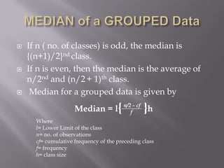
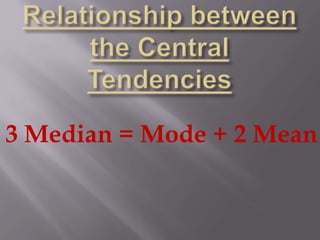
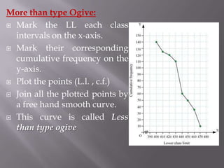
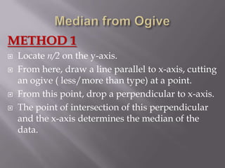

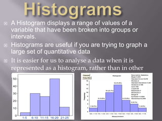
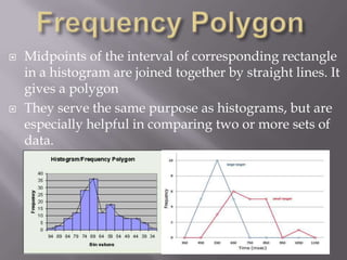
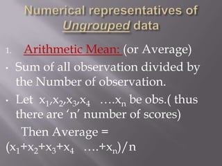
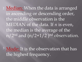
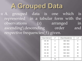
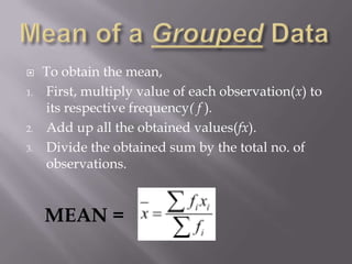
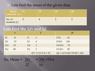
This document discusses various statistical concepts taught in 9th grade including histograms, frequency polygons, and numerical representatives of ungrouped data. It then introduces concepts related to grouped data such as calculating the mean, median, and mode of grouped data using different methods like the direct method, assumed mean method, and step deviation method. It also discusses the concepts of cumulative frequency, ogives (cumulative frequency curves), and how to find the median from an ogive.


![MEASURES-OF-CENTRAL-TENDENCIES-1[1] [Autosaved].pptx](https://cdn.slidesharecdn.com/ss_thumbnails/measures-of-central-tendencies-11autosaved-220906145428-d730d0eb-thumbnail.jpg?width=640&height=640&fit=bounds)


