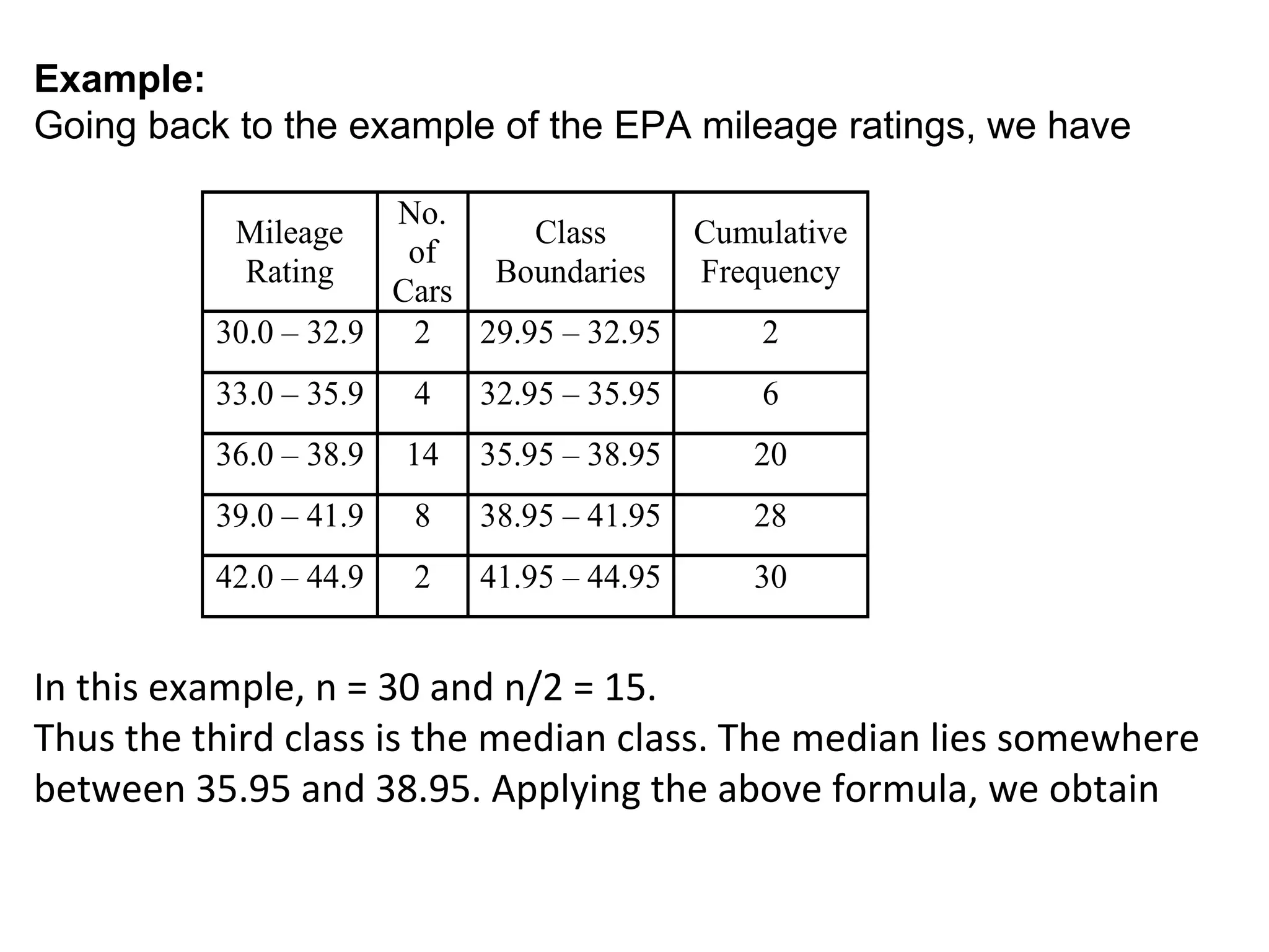
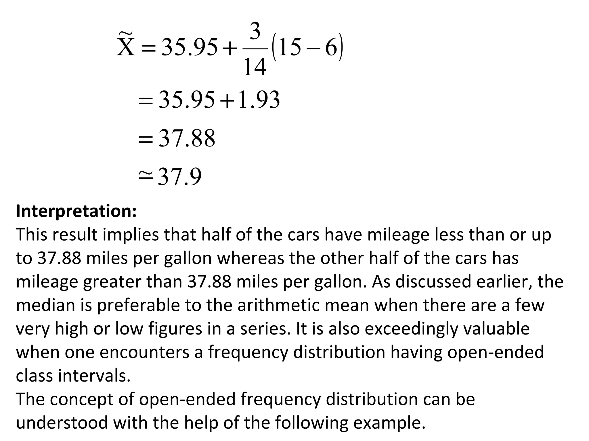
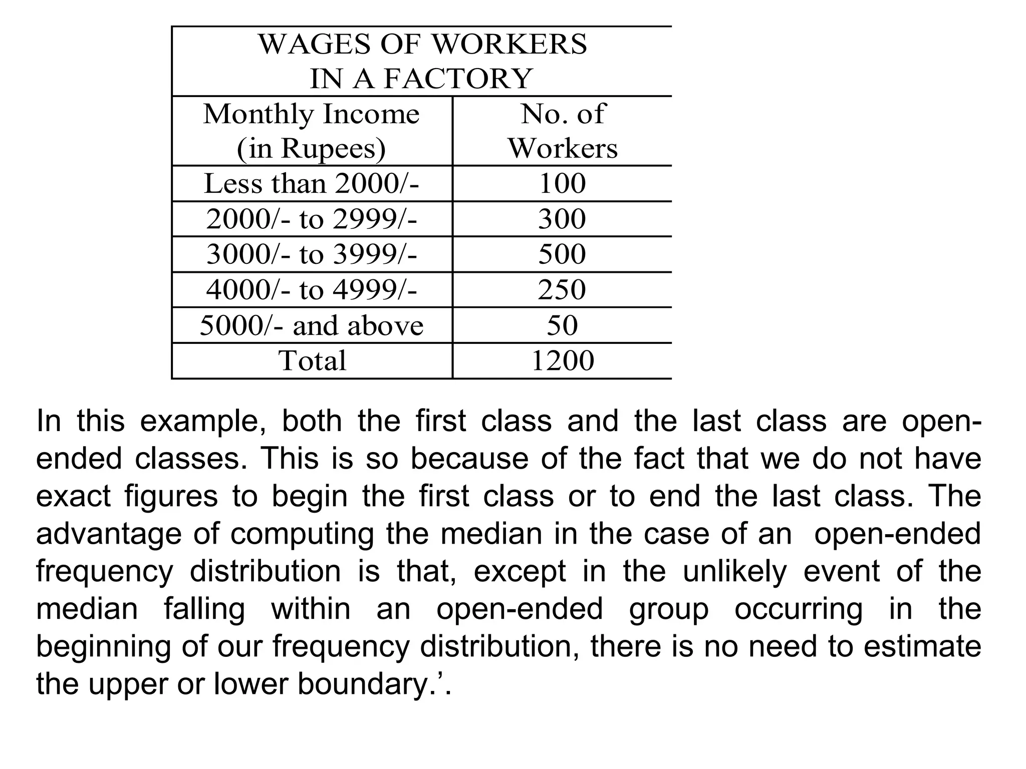
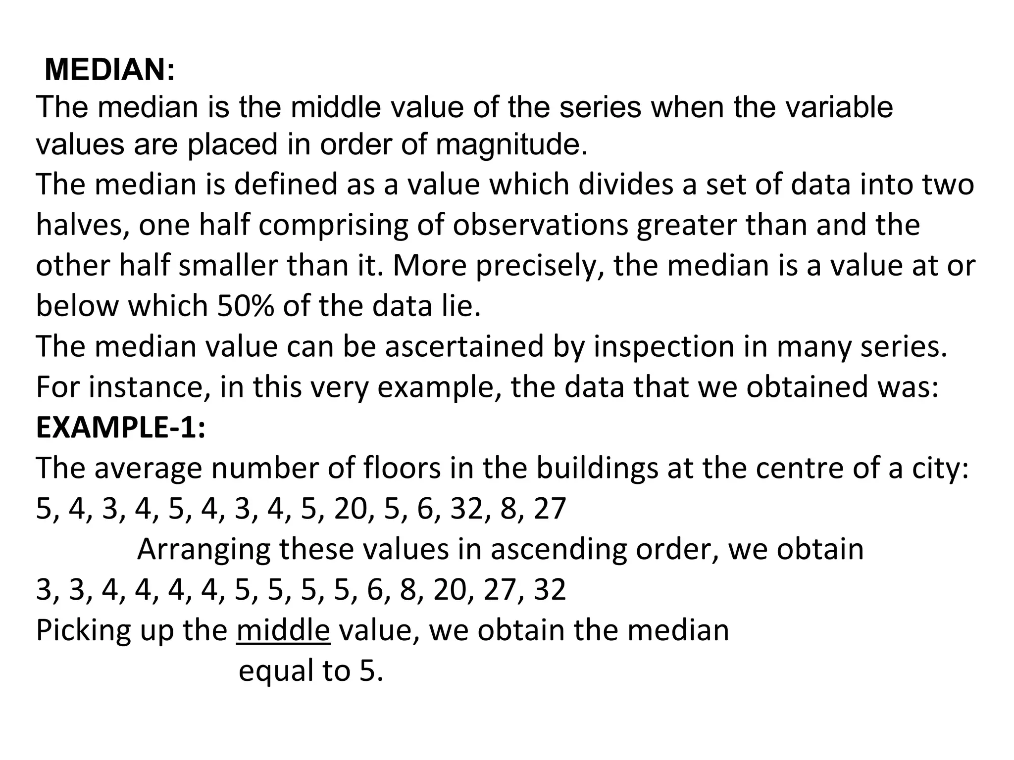
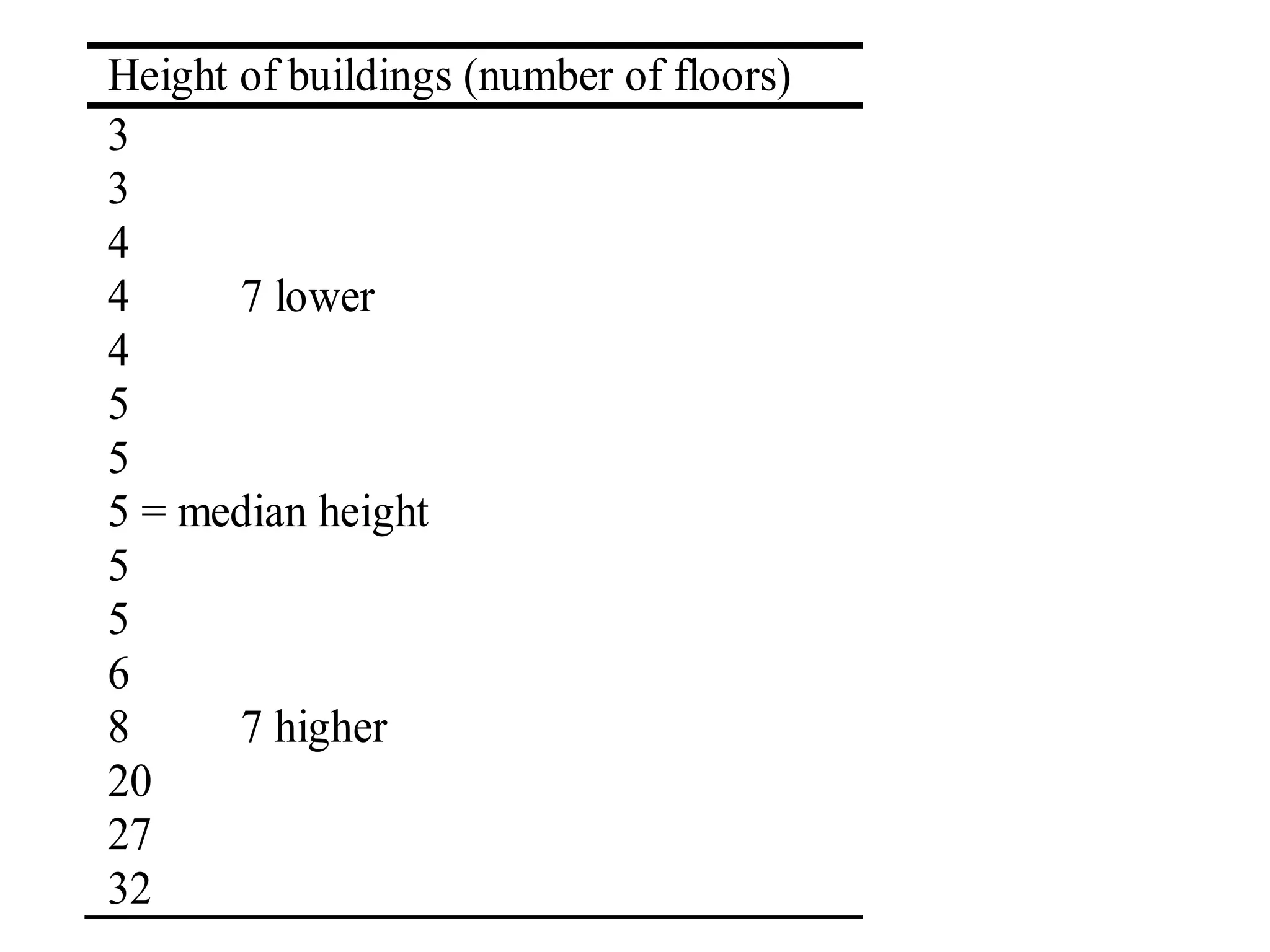
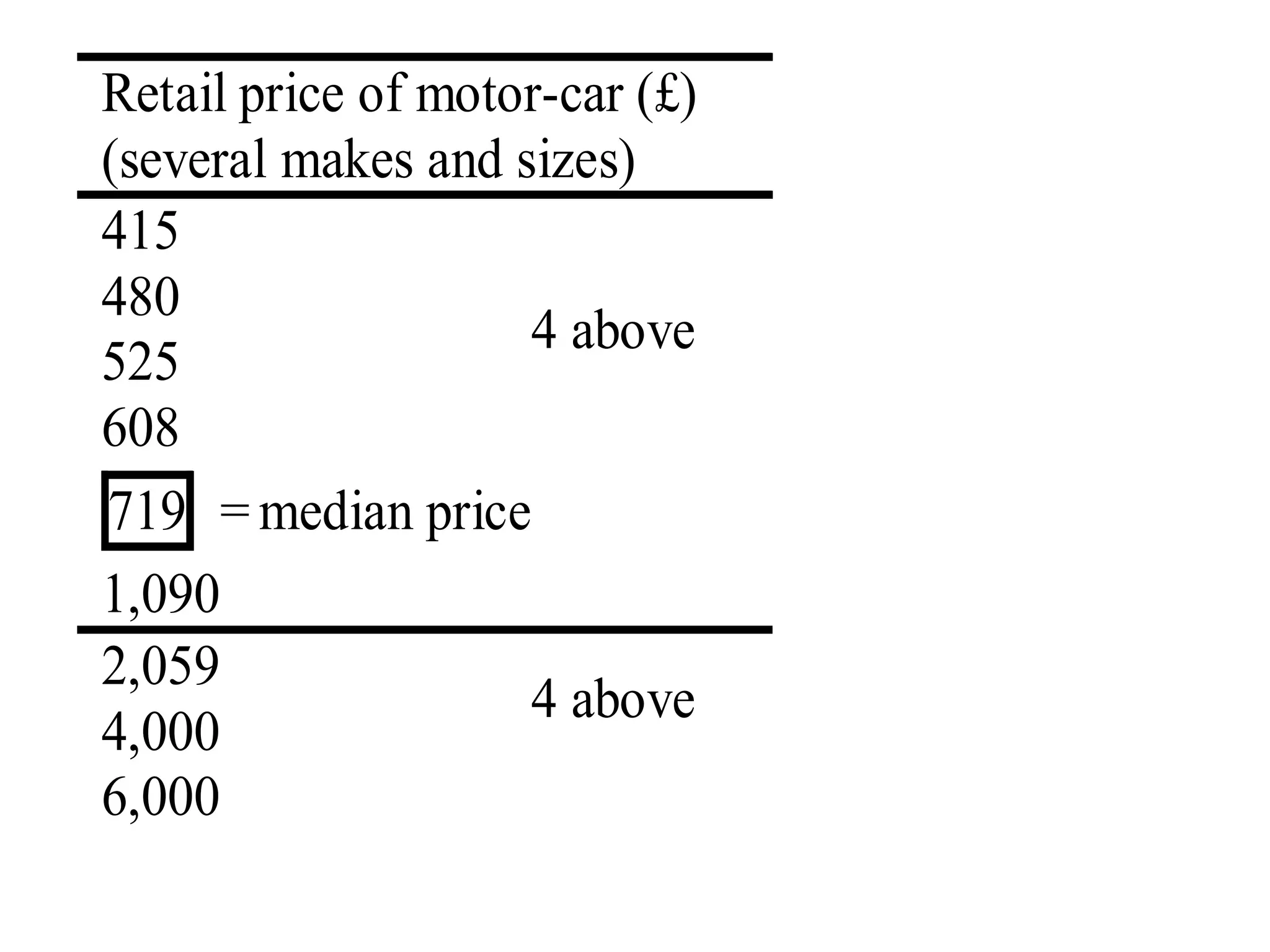
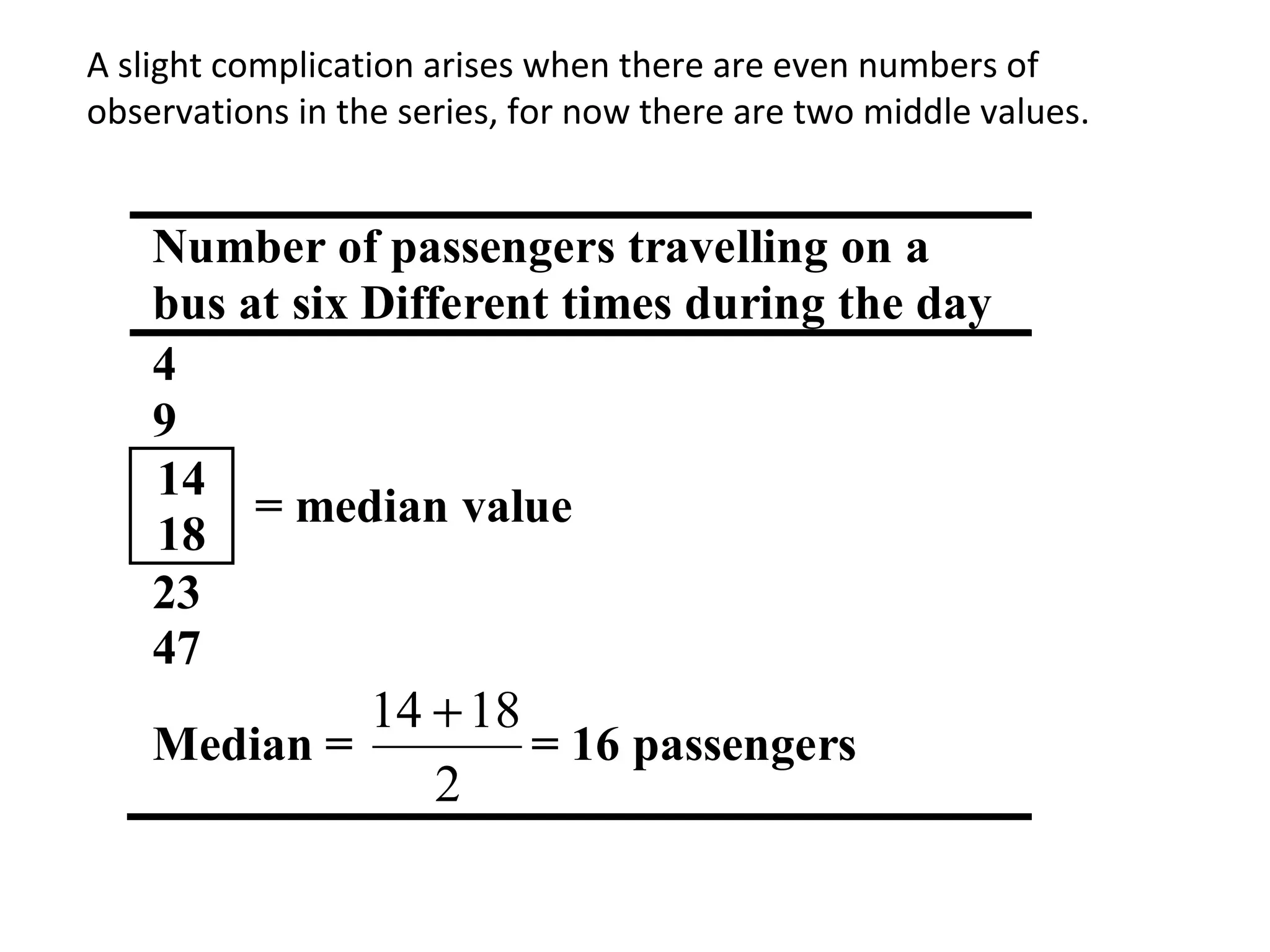
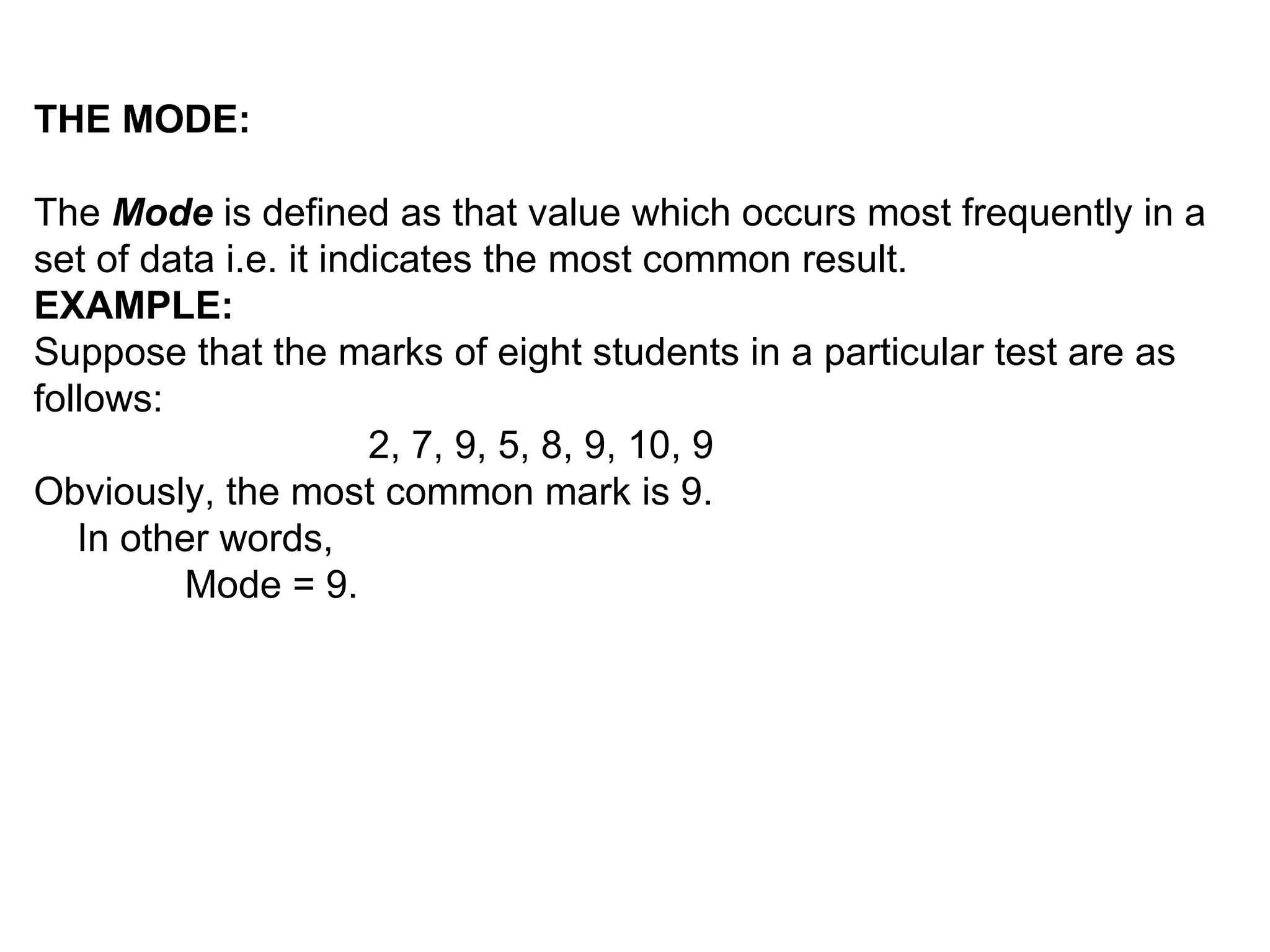
SlideShare a Scribd company logo
1 of 30
MEDIAN:
The median is the middle value of the series when the variable
values are placed in order of magnitude.
The median is defined as a value which divides a set of data into two
halves, one half comprising of observations greater than and the
other half smaller than it. More precisely, the median is a value at or
below which 50% of the data lie.
The median value can be ascertained by inspection in many series.
For instance, in this very example, the data that we obtained was:
EXAMPLE-1:
The average number of floors in the buildings at the centre of a city:
5, 4, 3, 4, 5, 4, 3, 4, 5, 20, 5, 6, 32, 8, 27
         Arranging these values in ascending order, we obtain
3, 3, 4, 4, 4, 4, 5, 5, 5, 5, 6, 8, 20, 27, 32
Picking up the middle value, we obtain the median
                  equal to 5.
Interpretation:
The median number of floors is 5. Out of those 15 buildings, 7 have
upto 5 floors and 7 have 5 floors or more. We noticed earlier that
the arithmetic mean was distorted toward the few extremely high
values in the series and hence became unrepresentative. The
median = 5 is much more representative of this series.
Height of buildings (number of floors)
3
3
4
4      7 lower
4
5
5
5 = median height
5
5
6
8      7 higher
20
27
32
Retail price of motor-car (£)
(several makes and sizes)
415
480
                    4 above
525
608
719 = median price
1,090
2,059
                    4 above
4,000
6,000
A slight complication arises when there are even numbers of
observations in the series, for now there are two middle values.


    Number of passengers travelling on a
    bus at six Different times during the day
    4
    9
    14
         = median value
    18
    23
    47
             14 + 18
    Median =         = 16 passengers
                2
Median in Case of a Frequency Distribution of a Continuous
Variable:

In case of a frequency distribution, the median is given by the
formula

                 ~      hn 
                 X = l +  − c
Where
                        f 2 
l =lower class boundary of the median class (i.e. that class for which
the cumulative frequency is just in excess of n/2).
h=class interval size of the median class
f =frequency of the median class
n=Σf (the total number of observations)
c =cumulative frequency of the class preceding the median class
Example:
Going back to the example of the EPA mileage ratings, we have

                      No.
           Mileage           Class    Cumulative
                       of
           Rating          Boundaries Frequency
                      Cars
          30.0 – 32.9 2 29.95 – 32.95     2
          33.0 – 35.9   4    32.95 – 35.95   6
          36.0 – 38.9   14   35.95 – 38.95   20
          39.0 – 41.9   8    38.95 – 41.95   28
          42.0 – 44.9   2    41.95 – 44.95   30


In this example, n = 30 and n/2 = 15.
Thus the third class is the median class. The median lies somewhere
between 35.95 and 38.95. Applying the above formula, we obtain
~            3
            X = 35.95 + (15 − 6 )
                        14
              = 35.95 + 1.93
              = 37.88
              ~ 37.9
              −
Interpretation:
This result implies that half of the cars have mileage less than or up
to 37.88 miles per gallon whereas the other half of the cars has
mileage greater than 37.88 miles per gallon. As discussed earlier, the
median is preferable to the arithmetic mean when there are a few
very high or low figures in a series. It is also exceedingly valuable
when one encounters a frequency distribution having open-ended
class intervals.
The concept of open-ended frequency distribution can be
understood with the help of the following example.
WAGES OF WORKERS
                   IN A FACTORY
           Monthly Income     No. of
             (in Rupees)      Workers
           Less than 2000/-     100
           2000/- to 2999/-     300
           3000/- to 3999/-     500
           4000/- to 4999/-     250
           5000/- and above      50
                 Total         1200

In this example, both the first class and the last class are open-
ended classes. This is so because of the fact that we do not have
exact figures to begin the first class or to end the last class. The
advantage of computing the median in the case of an open-ended
frequency distribution is that, except in the unlikely event of the
median falling within an open-ended group occurring in the
beginning of our frequency distribution, there is no need to estimate
the upper or lower boundary.’.
This is so because of the fact that, if the median is falling in an
intermediate class, then, obviously, the first class is not being
involved in its computation.The next concept that we will discuss is
the empirical relation between the mean, median and the mode.
This is a concept which is not based on a rigid mathematical
formula; rather, it is based on observation. In fact, the word
‘empirical’ implies ‘based on observation
QUARTILES
    The quartiles, together with the median, achieve the division of the total
area into four equal parts.
    The first, second and third quartiles are given by the formulae:

    First quartile:


                                h      n   
                       Q1 = l +         − c
                                f      4   
    Second quartile (i.e. median):

                              h  2n       h
                      Q2 = l +  − c  = l + ( n 2 − c )
                               f 4        f
Third quartile:


                  h 3n    
           Q3 =l +     −c 
                  f 4     

            f


                  25% 25% 25% 25%
                             ~      X
                    Q 1 Q2 = X Q3
The deciles and the percentiles given the division of the total area
into 10 and 100 equal parts respectively.


                          h n   
                  D1 = l +  − c 
                          f  10 

                          h  2n 
                  D2 = l +  − c 
                          f  10 


                          h  3n    
                  D3 = l +      −c 
                          f  10    
h n      
P1 = l +      − c
        f  100 

           h  2n    
   P2 = l +      − c
           f  100 
Again, it is easily seen that the 50th percentile is the same as the median,
the 25th percentile is the same as the 1st quartile, the 75th percentile is the
same as the 3rd quartile, the 40th percentile is the same as the 4th decile,
and so on.
         All these measures i.e. the median, quartiles, deciles and
percentiles are collectively called quantiles.       The question is, “What is
the significance of this concept of partitioning? Why is it that we wish to
divide our frequency distribution into two, four, ten or hundred parts?”
The answer to the above questions is: In certain situations, we may be
interested in describing the relative quantitative location of a particular
measurement within a data set. Quantiles provide us with an easy way of
achieving this. Out of these various quantiles, one of the most frequently
used is percentile ranking.
THE MODE:

The Mode is defined as that value which occurs most frequently in a
set of data i.e. it indicates the most common result.
EXAMPLE:
Suppose that the marks of eight students in a particular test are as
follows:
                       2, 7, 9, 5, 8, 9, 10, 9
Obviously, the most common mark is 9.
   In other words,
         Mode = 9.
THE MODE IN CASE OF THE FREQUENCY DISTRIBUTION OF A
CONTINUOUS VARIABLE:
In case of grouped data, the modal group is easily recognizable (the
one that has the highest frequency).
At what point within the modal group does the mode lie?
The answer is contained in the following formula:

 Mode:


          ˆ              f m − f1
          X = 1+                           xh
                 ( fm − f1 ) + ( fm − f2 )
ˆ              f m − f1
           X = 1+                           xh
                  ( fm − f1 ) + ( fm − f2 )
Where
l     = lower class boundary of the modal class,
fm    = frequency of the modal class,
f1    = frequency of the class preceding the
        modal class,
f2    = frequency of the class following modal
        class, and
h     = length of class interval of the modal class
Class Boundaries     No. of Cars
       Mileage Rating
          30.0 – 32.9         29.95 – 32.95           2
          33.0 – 35.9         32.95 – 35.95         4 = f1
          36.0 – 38.9         35.95 – 38.95        14 = fm
          39.0 – 41.9         38.95 – 41.95         8 = f2
          42.0 – 44.9         41.95 – 44.95           2

It is evident that the third class is the modal class.
The mode lies somewhere between 35.95 and 38.95.
In order to apply the formula for the mode, we note that
fm = 14, f1 = 4 and f2 = 8.
          ˆ                      14 −  4
          X         = .95 +
                     35                      ×3
                           (14 −4 ) + 14 − )
                                      (   8
                             10
                    = .95 +
                     35           × 3
                           10 + 6
                    = .95 + .875
                     35    1
                    = .825
                     37
DESIRABLE PROPERTIES OF THE MODE:
    •The mode is easily understood and easily ascertained in case of a
discrete frequency distribution.
    •It is not affected by a few very high or low values.
    The question arises, “When should we use the mode?”
    The answer to this question is that the mode is a valuable concept in
certain situations such as the one described below:
    Suppose the manager of a men’s clothing store is asked about the
average size of hats sold. He will probably think not of the arithmetic or
geometric mean size, or indeed the median size. Instead, he will in all
likelihood quote that particular size which is sold most often. This average
is of far more use to him as a businessman than the arithmetic mean,
geometric mean or the median. The modal size of all clothing is the size
which the businessman must stock in the greatest quantity and variety in
comparison with other sizes. Indeed, in most inventory (stock level)
problems, one needs the mode more often than any other measure of central
tendency. It should be noted that in some situations there may be no mode in
a simple series where no value occurs more than once.
Measures of Variability
Consider the following two data sets.
Set I: 1, 2, 3, 4, 5, 6, 6, 7, 8, 9, 10, 11
Set II: 4, 5, 5, 5, 6, 6, 6, 6, 7, 7, 7, 8

Compute the mean, median, and mode of each of the two data sets. As
you see from your results, the two data sets have the same mean, the same
median, and the same mode, all equal to 6. The two data sets also happen
to have the same number of observations, n =12. But the two data sets are
different. What is the main difference between them?
Figure shows data sets I and II. The two data sets have the same central
tendency, but they have a different variability. In particular, we see that
data set I is more variable than data set II. The values in set I are more
spread out: they lie farther away from their mean than do those of set II.
Short cut Formula for variance and Standard deviation


              x 2  x 2 
             ∑
         δ =
          2
                   ∑  
                  −    
              n
                   n  
         and
              x 2  x 2 
             ∑
          S=      ∑  
                  −    
              n
                   n  
Life (in
                No. of Bulbs   Mid-point
 Hundreds of                                 fx       fx2
                      f           x
   Hours)
      0–5             4           2.5       10.0      25.0
     5 – 10           9           7.5       67.5     506.25
    10 – 20           38         15.0      570.0     8550.0
    20 – 40           33         30.0      990.0    29700.0
  40 and over         16         50.0      800.0    40000.0
                      100                  2437.5   78781.25

      fx 2                         78781.25  2437.5  2 
     ∑       ∑ fx  
                    2
                                                           
  S=      −                  S=          −         
       n     n                    100
                                               100      
     
                  
=13.9 hundred hours
= 1390 hours
Coefficient of S.D:
The coefficient of variation CV describes
the standard deviation as a percent of the mean.
            S tan dand Deviation
       CV =                      ×100
                    Mean


                      The table at the left shows the heights (in
                      inches) and weights (in pounds) of the
                      members of a basketball team. Find the
                      coefficient of variation for each data set.
                      What can you conclude?
Median and mode

More Related Content

What's hot

Normal Distribution
Normal DistributionNormal Distribution
Normal DistributionCIToolkit
 
Lecture slides stats1.13.l09.air
Lecture slides stats1.13.l09.airLecture slides stats1.13.l09.air
Lecture slides stats1.13.l09.airatutor_te
 
Measures of central tendency
Measures of central tendency Measures of central tendency
Measures of central tendency Jagdish Powar
 
Measures of dispersion
Measures of dispersionMeasures of dispersion
Measures of dispersionSachin Shekde
 
Correlation Coefficient
Correlation CoefficientCorrelation Coefficient
Correlation CoefficientSaadSaif6
 
quartile deviation: An introduction
quartile deviation: An introductionquartile deviation: An introduction
quartile deviation: An introductionDr Rajesh Verma
 
Correlation and regression
Correlation and regressionCorrelation and regression
Correlation and regressionAbdelaziz Tayoun
 
Correlation and regression
Correlation and regressionCorrelation and regression
Correlation and regressionMOHIT PANCHAL
 
Measures of central tendency
Measures of central tendencyMeasures of central tendency
Measures of central tendencyChie Pegollo
 
Anova ONE WAY
Anova ONE WAYAnova ONE WAY
Anova ONE WAYelulu123
 

What's hot (20)

Normal Distribution
Normal DistributionNormal Distribution
Normal Distribution
 
Mann Whitney U test
Mann Whitney U testMann Whitney U test
Mann Whitney U test
 
Lecture slides stats1.13.l09.air
Lecture slides stats1.13.l09.airLecture slides stats1.13.l09.air
Lecture slides stats1.13.l09.air
 
Measures of central tendency
Measures of central tendency Measures of central tendency
Measures of central tendency
 
Measures of dispersion
Measures of dispersionMeasures of dispersion
Measures of dispersion
 
Cumulative Frequency
Cumulative FrequencyCumulative Frequency
Cumulative Frequency
 
Correlation Coefficient
Correlation CoefficientCorrelation Coefficient
Correlation Coefficient
 
quartile deviation: An introduction
quartile deviation: An introductionquartile deviation: An introduction
quartile deviation: An introduction
 
Correlation and regression
Correlation and regressionCorrelation and regression
Correlation and regression
 
Frequency distribution
Frequency distributionFrequency distribution
Frequency distribution
 
8. Correlation
8. Correlation8. Correlation
8. Correlation
 
Estimating a Population Proportion
Estimating a Population Proportion  Estimating a Population Proportion
Estimating a Population Proportion
 
Kruskal wallis test
Kruskal wallis testKruskal wallis test
Kruskal wallis test
 
Confidence Intervals
Confidence IntervalsConfidence Intervals
Confidence Intervals
 
Correlation and regression
Correlation and regressionCorrelation and regression
Correlation and regression
 
Median & mode
Median & modeMedian & mode
Median & mode
 
Measures of central tendency
Measures of central tendencyMeasures of central tendency
Measures of central tendency
 
Anova ONE WAY
Anova ONE WAYAnova ONE WAY
Anova ONE WAY
 
The Normal Distribution
The Normal DistributionThe Normal Distribution
The Normal Distribution
 
Measure of central tendency
Measure of central tendencyMeasure of central tendency
Measure of central tendency
 

Similar to Median and mode

Quartiles, Deciles and Percentiles
Quartiles, Deciles and PercentilesQuartiles, Deciles and Percentiles
Quartiles, Deciles and PercentilesMuhammad Amir Sohail
 
Biostatistics and Research Methodology: Unit I - Measures of Central Tendency...
Biostatistics and Research Methodology: Unit I - Measures of Central Tendency...Biostatistics and Research Methodology: Unit I - Measures of Central Tendency...
Biostatistics and Research Methodology: Unit I - Measures of Central Tendency...Chaitali Dongaonkar
 
Importance of The non-modal and the bi-modal situation,(simple) arithmetic me...
Importance of The non-modal and the bi-modal situation,(simple) arithmetic me...Importance of The non-modal and the bi-modal situation,(simple) arithmetic me...
Importance of The non-modal and the bi-modal situation,(simple) arithmetic me...Osama Yousaf
 
Central tendency
Central tendencyCentral tendency
Central tendencyvnkatare
 
Group 3 measures of central tendency and variation - (mean, median, mode, ra...
Group 3  measures of central tendency and variation - (mean, median, mode, ra...Group 3  measures of central tendency and variation - (mean, median, mode, ra...
Group 3 measures of central tendency and variation - (mean, median, mode, ra...reymartyvette_0611
 
MEASURES-OF-CENTRAL-TENDENCY-lecture-edited.pptx
MEASURES-OF-CENTRAL-TENDENCY-lecture-edited.pptxMEASURES-OF-CENTRAL-TENDENCY-lecture-edited.pptx
MEASURES-OF-CENTRAL-TENDENCY-lecture-edited.pptxJhayMarkMaltoLacsam
 
Measures of central tendency
Measures of central tendencyMeasures of central tendency
Measures of central tendencyManu Antony
 
Analysis and interpretation of Assessment.pptx
Analysis and interpretation of Assessment.pptxAnalysis and interpretation of Assessment.pptx
Analysis and interpretation of Assessment.pptxAeonneFlux
 
Statistics Math project class 10th
Statistics Math project class 10thStatistics Math project class 10th
Statistics Math project class 10thRiya Singh
 
CLASS 10 MEAN MEDIAN MODE
CLASS 10 MEAN MEDIAN MODECLASS 10 MEAN MEDIAN MODE
CLASS 10 MEAN MEDIAN MODEAKBAR1961
 
MEASURES-OF-CENTRAL-TENDENCIES-1[1] [Autosaved].pptx
MEASURES-OF-CENTRAL-TENDENCIES-1[1] [Autosaved].pptxMEASURES-OF-CENTRAL-TENDENCIES-1[1] [Autosaved].pptx
MEASURES-OF-CENTRAL-TENDENCIES-1[1] [Autosaved].pptxamadapaulo
 
Unit 1 - Measures of Dispersion - 18MAB303T - PPT - Part 2.pdf
Unit 1 - Measures of Dispersion - 18MAB303T - PPT - Part 2.pdfUnit 1 - Measures of Dispersion - 18MAB303T - PPT - Part 2.pdf
Unit 1 - Measures of Dispersion - 18MAB303T - PPT - Part 2.pdfAravindS199
 
measures of centraltendency.ppt
measures of centraltendency.pptmeasures of centraltendency.ppt
measures of centraltendency.pptSoujanyaLk1
 

Similar to Median and mode (20)

Measure of mode in biostatic
Measure of mode in biostaticMeasure of mode in biostatic
Measure of mode in biostatic
 
Quartiles, Deciles and Percentiles
Quartiles, Deciles and PercentilesQuartiles, Deciles and Percentiles
Quartiles, Deciles and Percentiles
 
Biostatistics and Research Methodology: Unit I - Measures of Central Tendency...
Biostatistics and Research Methodology: Unit I - Measures of Central Tendency...Biostatistics and Research Methodology: Unit I - Measures of Central Tendency...
Biostatistics and Research Methodology: Unit I - Measures of Central Tendency...
 
Importance of The non-modal and the bi-modal situation,(simple) arithmetic me...
Importance of The non-modal and the bi-modal situation,(simple) arithmetic me...Importance of The non-modal and the bi-modal situation,(simple) arithmetic me...
Importance of The non-modal and the bi-modal situation,(simple) arithmetic me...
 
STATISTICS AND PROBABILITY.pptx
STATISTICS AND PROBABILITY.pptxSTATISTICS AND PROBABILITY.pptx
STATISTICS AND PROBABILITY.pptx
 
Central tendency
Central tendencyCentral tendency
Central tendency
 
Group 3 measures of central tendency and variation - (mean, median, mode, ra...
Group 3  measures of central tendency and variation - (mean, median, mode, ra...Group 3  measures of central tendency and variation - (mean, median, mode, ra...
Group 3 measures of central tendency and variation - (mean, median, mode, ra...
 
Mod mean quartile
Mod mean quartileMod mean quartile
Mod mean quartile
 
statistics 10th (1) (3).pdf
statistics 10th (1) (3).pdfstatistics 10th (1) (3).pdf
statistics 10th (1) (3).pdf
 
Measures of Variation
Measures of VariationMeasures of Variation
Measures of Variation
 
MEASURES-OF-CENTRAL-TENDENCY-lecture-edited.pptx
MEASURES-OF-CENTRAL-TENDENCY-lecture-edited.pptxMEASURES-OF-CENTRAL-TENDENCY-lecture-edited.pptx
MEASURES-OF-CENTRAL-TENDENCY-lecture-edited.pptx
 
Measures of central tendency
Measures of central tendencyMeasures of central tendency
Measures of central tendency
 
LECTURE NO 7.pdf
LECTURE NO 7.pdfLECTURE NO 7.pdf
LECTURE NO 7.pdf
 
Analysis and interpretation of Assessment.pptx
Analysis and interpretation of Assessment.pptxAnalysis and interpretation of Assessment.pptx
Analysis and interpretation of Assessment.pptx
 
Statistics Math project class 10th
Statistics Math project class 10thStatistics Math project class 10th
Statistics Math project class 10th
 
CLASS 10 MEAN MEDIAN MODE
CLASS 10 MEAN MEDIAN MODECLASS 10 MEAN MEDIAN MODE
CLASS 10 MEAN MEDIAN MODE
 
7. the t distribution
7. the t distribution7. the t distribution
7. the t distribution
 
MEASURES-OF-CENTRAL-TENDENCIES-1[1] [Autosaved].pptx
MEASURES-OF-CENTRAL-TENDENCIES-1[1] [Autosaved].pptxMEASURES-OF-CENTRAL-TENDENCIES-1[1] [Autosaved].pptx
MEASURES-OF-CENTRAL-TENDENCIES-1[1] [Autosaved].pptx
 
Unit 1 - Measures of Dispersion - 18MAB303T - PPT - Part 2.pdf
Unit 1 - Measures of Dispersion - 18MAB303T - PPT - Part 2.pdfUnit 1 - Measures of Dispersion - 18MAB303T - PPT - Part 2.pdf
Unit 1 - Measures of Dispersion - 18MAB303T - PPT - Part 2.pdf
 
measures of centraltendency.ppt
measures of centraltendency.pptmeasures of centraltendency.ppt
measures of centraltendency.ppt
 

Recently uploaded

Tech-Forward - Achieving Business Readiness For Copilot in Microsoft 365
Tech-Forward - Achieving Business Readiness For Copilot in Microsoft 365Tech-Forward - Achieving Business Readiness For Copilot in Microsoft 365
Tech-Forward - Achieving Business Readiness For Copilot in Microsoft 3652toLead Limited
 
08448380779 Call Girls In Greater Kailash - I Women Seeking Men
08448380779 Call Girls In Greater Kailash - I Women Seeking Men08448380779 Call Girls In Greater Kailash - I Women Seeking Men
08448380779 Call Girls In Greater Kailash - I Women Seeking MenDelhi Call girls
 
Artificial intelligence in the post-deep learning era
Artificial intelligence in the post-deep learning eraArtificial intelligence in the post-deep learning era
Artificial intelligence in the post-deep learning eraDeakin University
 
Slack Application Development 101 Slides
Slack Application Development 101 SlidesSlack Application Development 101 Slides
Slack Application Development 101 Slidespraypatel2
 
Benefits Of Flutter Compared To Other Frameworks
Benefits Of Flutter Compared To Other FrameworksBenefits Of Flutter Compared To Other Frameworks
Benefits Of Flutter Compared To Other FrameworksSoftradix Technologies
 
08448380779 Call Girls In Diplomatic Enclave Women Seeking Men
08448380779 Call Girls In Diplomatic Enclave Women Seeking Men08448380779 Call Girls In Diplomatic Enclave Women Seeking Men
08448380779 Call Girls In Diplomatic Enclave Women Seeking MenDelhi Call girls
 
SIEMENS: RAPUNZEL – A Tale About Knowledge Graph
SIEMENS: RAPUNZEL – A Tale About Knowledge GraphSIEMENS: RAPUNZEL – A Tale About Knowledge Graph
SIEMENS: RAPUNZEL – A Tale About Knowledge GraphNeo4j
 
FULL ENJOY 🔝 8264348440 🔝 Call Girls in Diplomatic Enclave | Delhi
FULL ENJOY 🔝 8264348440 🔝 Call Girls in Diplomatic Enclave | DelhiFULL ENJOY 🔝 8264348440 🔝 Call Girls in Diplomatic Enclave | Delhi
FULL ENJOY 🔝 8264348440 🔝 Call Girls in Diplomatic Enclave | Delhisoniya singh
 
Kotlin Multiplatform & Compose Multiplatform - Starter kit for pragmatics
Kotlin Multiplatform & Compose Multiplatform - Starter kit for pragmaticsKotlin Multiplatform & Compose Multiplatform - Starter kit for pragmatics
Kotlin Multiplatform & Compose Multiplatform - Starter kit for pragmaticscarlostorres15106
 
Transforming Data Streams with Kafka Connect: An Introduction to Single Messa...
Transforming Data Streams with Kafka Connect: An Introduction to Single Messa...Transforming Data Streams with Kafka Connect: An Introduction to Single Messa...
Transforming Data Streams with Kafka Connect: An Introduction to Single Messa...HostedbyConfluent
 
Install Stable Diffusion in windows machine
Install Stable Diffusion in windows machineInstall Stable Diffusion in windows machine
Install Stable Diffusion in windows machinePadma Pradeep
 
GenCyber Cyber Security Day Presentation
GenCyber Cyber Security Day PresentationGenCyber Cyber Security Day Presentation
GenCyber Cyber Security Day PresentationMichael W. Hawkins
 
Maximizing Board Effectiveness 2024 Webinar.pptx
Maximizing Board Effectiveness 2024 Webinar.pptxMaximizing Board Effectiveness 2024 Webinar.pptx
Maximizing Board Effectiveness 2024 Webinar.pptxOnBoard
 
How to Remove Document Management Hurdles with X-Docs?
How to Remove Document Management Hurdles with X-Docs?How to Remove Document Management Hurdles with X-Docs?
How to Remove Document Management Hurdles with X-Docs?XfilesPro
 
CloudStudio User manual (basic edition):
CloudStudio User manual (basic edition):CloudStudio User manual (basic edition):
CloudStudio User manual (basic edition):comworks
 
SQL Database Design For Developers at php[tek] 2024
SQL Database Design For Developers at php[tek] 2024SQL Database Design For Developers at php[tek] 2024
SQL Database Design For Developers at php[tek] 2024Scott Keck-Warren
 
#StandardsGoals for 2024: What’s new for BISAC - Tech Forum 2024
#StandardsGoals for 2024: What’s new for BISAC - Tech Forum 2024#StandardsGoals for 2024: What’s new for BISAC - Tech Forum 2024
#StandardsGoals for 2024: What’s new for BISAC - Tech Forum 2024BookNet Canada
 
Hyderabad Call Girls Khairatabad ✨ 7001305949 ✨ Cheap Price Your Budget
Hyderabad Call Girls Khairatabad ✨ 7001305949 ✨ Cheap Price Your BudgetHyderabad Call Girls Khairatabad ✨ 7001305949 ✨ Cheap Price Your Budget
Hyderabad Call Girls Khairatabad ✨ 7001305949 ✨ Cheap Price Your BudgetEnjoy Anytime
 
The Codex of Business Writing Software for Real-World Solutions 2.pptx
The Codex of Business Writing Software for Real-World Solutions 2.pptxThe Codex of Business Writing Software for Real-World Solutions 2.pptx
The Codex of Business Writing Software for Real-World Solutions 2.pptxMalak Abu Hammad
 
Injustice - Developers Among Us (SciFiDevCon 2024)
Injustice - Developers Among Us (SciFiDevCon 2024)Injustice - Developers Among Us (SciFiDevCon 2024)
Injustice - Developers Among Us (SciFiDevCon 2024)Allon Mureinik
 

Recently uploaded (20)

Tech-Forward - Achieving Business Readiness For Copilot in Microsoft 365
Tech-Forward - Achieving Business Readiness For Copilot in Microsoft 365Tech-Forward - Achieving Business Readiness For Copilot in Microsoft 365
Tech-Forward - Achieving Business Readiness For Copilot in Microsoft 365
 
08448380779 Call Girls In Greater Kailash - I Women Seeking Men
08448380779 Call Girls In Greater Kailash - I Women Seeking Men08448380779 Call Girls In Greater Kailash - I Women Seeking Men
08448380779 Call Girls In Greater Kailash - I Women Seeking Men
 
Artificial intelligence in the post-deep learning era
Artificial intelligence in the post-deep learning eraArtificial intelligence in the post-deep learning era
Artificial intelligence in the post-deep learning era
 
Slack Application Development 101 Slides
Slack Application Development 101 SlidesSlack Application Development 101 Slides
Slack Application Development 101 Slides
 
Benefits Of Flutter Compared To Other Frameworks
Benefits Of Flutter Compared To Other FrameworksBenefits Of Flutter Compared To Other Frameworks
Benefits Of Flutter Compared To Other Frameworks
 
08448380779 Call Girls In Diplomatic Enclave Women Seeking Men
08448380779 Call Girls In Diplomatic Enclave Women Seeking Men08448380779 Call Girls In Diplomatic Enclave Women Seeking Men
08448380779 Call Girls In Diplomatic Enclave Women Seeking Men
 
SIEMENS: RAPUNZEL – A Tale About Knowledge Graph
SIEMENS: RAPUNZEL – A Tale About Knowledge GraphSIEMENS: RAPUNZEL – A Tale About Knowledge Graph
SIEMENS: RAPUNZEL – A Tale About Knowledge Graph
 
FULL ENJOY 🔝 8264348440 🔝 Call Girls in Diplomatic Enclave | Delhi
FULL ENJOY 🔝 8264348440 🔝 Call Girls in Diplomatic Enclave | DelhiFULL ENJOY 🔝 8264348440 🔝 Call Girls in Diplomatic Enclave | Delhi
FULL ENJOY 🔝 8264348440 🔝 Call Girls in Diplomatic Enclave | Delhi
 
Kotlin Multiplatform & Compose Multiplatform - Starter kit for pragmatics
Kotlin Multiplatform & Compose Multiplatform - Starter kit for pragmaticsKotlin Multiplatform & Compose Multiplatform - Starter kit for pragmatics
Kotlin Multiplatform & Compose Multiplatform - Starter kit for pragmatics
 
Transforming Data Streams with Kafka Connect: An Introduction to Single Messa...
Transforming Data Streams with Kafka Connect: An Introduction to Single Messa...Transforming Data Streams with Kafka Connect: An Introduction to Single Messa...
Transforming Data Streams with Kafka Connect: An Introduction to Single Messa...
 
Install Stable Diffusion in windows machine
Install Stable Diffusion in windows machineInstall Stable Diffusion in windows machine
Install Stable Diffusion in windows machine
 
GenCyber Cyber Security Day Presentation
GenCyber Cyber Security Day PresentationGenCyber Cyber Security Day Presentation
GenCyber Cyber Security Day Presentation
 
Maximizing Board Effectiveness 2024 Webinar.pptx
Maximizing Board Effectiveness 2024 Webinar.pptxMaximizing Board Effectiveness 2024 Webinar.pptx
Maximizing Board Effectiveness 2024 Webinar.pptx
 
How to Remove Document Management Hurdles with X-Docs?
How to Remove Document Management Hurdles with X-Docs?How to Remove Document Management Hurdles with X-Docs?
How to Remove Document Management Hurdles with X-Docs?
 
CloudStudio User manual (basic edition):
CloudStudio User manual (basic edition):CloudStudio User manual (basic edition):
CloudStudio User manual (basic edition):
 
SQL Database Design For Developers at php[tek] 2024
SQL Database Design For Developers at php[tek] 2024SQL Database Design For Developers at php[tek] 2024
SQL Database Design For Developers at php[tek] 2024
 
#StandardsGoals for 2024: What’s new for BISAC - Tech Forum 2024
#StandardsGoals for 2024: What’s new for BISAC - Tech Forum 2024#StandardsGoals for 2024: What’s new for BISAC - Tech Forum 2024
#StandardsGoals for 2024: What’s new for BISAC - Tech Forum 2024
 
Hyderabad Call Girls Khairatabad ✨ 7001305949 ✨ Cheap Price Your Budget
Hyderabad Call Girls Khairatabad ✨ 7001305949 ✨ Cheap Price Your BudgetHyderabad Call Girls Khairatabad ✨ 7001305949 ✨ Cheap Price Your Budget
Hyderabad Call Girls Khairatabad ✨ 7001305949 ✨ Cheap Price Your Budget
 
The Codex of Business Writing Software for Real-World Solutions 2.pptx
The Codex of Business Writing Software for Real-World Solutions 2.pptxThe Codex of Business Writing Software for Real-World Solutions 2.pptx
The Codex of Business Writing Software for Real-World Solutions 2.pptx
 
Injustice - Developers Among Us (SciFiDevCon 2024)
Injustice - Developers Among Us (SciFiDevCon 2024)Injustice - Developers Among Us (SciFiDevCon 2024)
Injustice - Developers Among Us (SciFiDevCon 2024)
 

Median and mode

  • 1. MEDIAN: The median is the middle value of the series when the variable values are placed in order of magnitude. The median is defined as a value which divides a set of data into two halves, one half comprising of observations greater than and the other half smaller than it. More precisely, the median is a value at or below which 50% of the data lie. The median value can be ascertained by inspection in many series. For instance, in this very example, the data that we obtained was: EXAMPLE-1: The average number of floors in the buildings at the centre of a city: 5, 4, 3, 4, 5, 4, 3, 4, 5, 20, 5, 6, 32, 8, 27 Arranging these values in ascending order, we obtain 3, 3, 4, 4, 4, 4, 5, 5, 5, 5, 6, 8, 20, 27, 32 Picking up the middle value, we obtain the median equal to 5.
  • 2. Interpretation: The median number of floors is 5. Out of those 15 buildings, 7 have upto 5 floors and 7 have 5 floors or more. We noticed earlier that the arithmetic mean was distorted toward the few extremely high values in the series and hence became unrepresentative. The median = 5 is much more representative of this series.
  • 3. Height of buildings (number of floors) 3 3 4 4 7 lower 4 5 5 5 = median height 5 5 6 8 7 higher 20 27 32
  • 4. Retail price of motor-car (£) (several makes and sizes) 415 480 4 above 525 608 719 = median price 1,090 2,059 4 above 4,000 6,000
  • 5. A slight complication arises when there are even numbers of observations in the series, for now there are two middle values. Number of passengers travelling on a bus at six Different times during the day 4 9 14 = median value 18 23 47 14 + 18 Median = = 16 passengers 2
  • 6. Median in Case of a Frequency Distribution of a Continuous Variable: In case of a frequency distribution, the median is given by the formula ~ hn  X = l +  − c Where f 2  l =lower class boundary of the median class (i.e. that class for which the cumulative frequency is just in excess of n/2). h=class interval size of the median class f =frequency of the median class n=Σf (the total number of observations) c =cumulative frequency of the class preceding the median class
  • 7. Example: Going back to the example of the EPA mileage ratings, we have No. Mileage Class Cumulative of Rating Boundaries Frequency Cars 30.0 – 32.9 2 29.95 – 32.95 2 33.0 – 35.9 4 32.95 – 35.95 6 36.0 – 38.9 14 35.95 – 38.95 20 39.0 – 41.9 8 38.95 – 41.95 28 42.0 – 44.9 2 41.95 – 44.95 30 In this example, n = 30 and n/2 = 15. Thus the third class is the median class. The median lies somewhere between 35.95 and 38.95. Applying the above formula, we obtain
  • 8. ~ 3 X = 35.95 + (15 − 6 ) 14 = 35.95 + 1.93 = 37.88 ~ 37.9 − Interpretation: This result implies that half of the cars have mileage less than or up to 37.88 miles per gallon whereas the other half of the cars has mileage greater than 37.88 miles per gallon. As discussed earlier, the median is preferable to the arithmetic mean when there are a few very high or low figures in a series. It is also exceedingly valuable when one encounters a frequency distribution having open-ended class intervals. The concept of open-ended frequency distribution can be understood with the help of the following example.
  • 9. WAGES OF WORKERS IN A FACTORY Monthly Income No. of (in Rupees) Workers Less than 2000/- 100 2000/- to 2999/- 300 3000/- to 3999/- 500 4000/- to 4999/- 250 5000/- and above 50 Total 1200 In this example, both the first class and the last class are open- ended classes. This is so because of the fact that we do not have exact figures to begin the first class or to end the last class. The advantage of computing the median in the case of an open-ended frequency distribution is that, except in the unlikely event of the median falling within an open-ended group occurring in the beginning of our frequency distribution, there is no need to estimate the upper or lower boundary.’.
  • 10. This is so because of the fact that, if the median is falling in an intermediate class, then, obviously, the first class is not being involved in its computation.The next concept that we will discuss is the empirical relation between the mean, median and the mode. This is a concept which is not based on a rigid mathematical formula; rather, it is based on observation. In fact, the word ‘empirical’ implies ‘based on observation
  • 11. QUARTILES The quartiles, together with the median, achieve the division of the total area into four equal parts. The first, second and third quartiles are given by the formulae: First quartile: h n  Q1 = l +  − c f 4  Second quartile (i.e. median): h  2n  h Q2 = l +  − c  = l + ( n 2 − c ) f 4  f
  • 12. Third quartile: h 3n  Q3 =l +  −c  f 4  f 25% 25% 25% 25% ~ X Q 1 Q2 = X Q3
  • 13. The deciles and the percentiles given the division of the total area into 10 and 100 equal parts respectively. h n  D1 = l +  − c  f  10  h  2n  D2 = l +  − c  f  10  h  3n  D3 = l +  −c  f  10 
  • 14. h n  P1 = l +  − c f  100  h  2n  P2 = l +  − c f  100 
  • 15. Again, it is easily seen that the 50th percentile is the same as the median, the 25th percentile is the same as the 1st quartile, the 75th percentile is the same as the 3rd quartile, the 40th percentile is the same as the 4th decile, and so on. All these measures i.e. the median, quartiles, deciles and percentiles are collectively called quantiles. The question is, “What is the significance of this concept of partitioning? Why is it that we wish to divide our frequency distribution into two, four, ten or hundred parts?” The answer to the above questions is: In certain situations, we may be interested in describing the relative quantitative location of a particular measurement within a data set. Quantiles provide us with an easy way of achieving this. Out of these various quantiles, one of the most frequently used is percentile ranking.
  • 16. THE MODE: The Mode is defined as that value which occurs most frequently in a set of data i.e. it indicates the most common result. EXAMPLE: Suppose that the marks of eight students in a particular test are as follows: 2, 7, 9, 5, 8, 9, 10, 9 Obviously, the most common mark is 9. In other words, Mode = 9.
  • 17. THE MODE IN CASE OF THE FREQUENCY DISTRIBUTION OF A CONTINUOUS VARIABLE: In case of grouped data, the modal group is easily recognizable (the one that has the highest frequency). At what point within the modal group does the mode lie? The answer is contained in the following formula: Mode: ˆ f m − f1 X = 1+ xh ( fm − f1 ) + ( fm − f2 )
  • 18. ˆ f m − f1 X = 1+ xh ( fm − f1 ) + ( fm − f2 ) Where l = lower class boundary of the modal class, fm = frequency of the modal class, f1 = frequency of the class preceding the modal class, f2 = frequency of the class following modal class, and h = length of class interval of the modal class
  • 19. Class Boundaries No. of Cars Mileage Rating 30.0 – 32.9 29.95 – 32.95 2 33.0 – 35.9 32.95 – 35.95 4 = f1 36.0 – 38.9 35.95 – 38.95 14 = fm 39.0 – 41.9 38.95 – 41.95 8 = f2 42.0 – 44.9 41.95 – 44.95 2 It is evident that the third class is the modal class. The mode lies somewhere between 35.95 and 38.95. In order to apply the formula for the mode, we note that fm = 14, f1 = 4 and f2 = 8. ˆ 14 − 4 X = .95 + 35 ×3 (14 −4 ) + 14 − ) ( 8 10 = .95 + 35 × 3 10 + 6 = .95 + .875 35 1 = .825 37
  • 20. DESIRABLE PROPERTIES OF THE MODE: •The mode is easily understood and easily ascertained in case of a discrete frequency distribution. •It is not affected by a few very high or low values. The question arises, “When should we use the mode?” The answer to this question is that the mode is a valuable concept in certain situations such as the one described below: Suppose the manager of a men’s clothing store is asked about the average size of hats sold. He will probably think not of the arithmetic or geometric mean size, or indeed the median size. Instead, he will in all likelihood quote that particular size which is sold most often. This average is of far more use to him as a businessman than the arithmetic mean, geometric mean or the median. The modal size of all clothing is the size which the businessman must stock in the greatest quantity and variety in comparison with other sizes. Indeed, in most inventory (stock level) problems, one needs the mode more often than any other measure of central tendency. It should be noted that in some situations there may be no mode in a simple series where no value occurs more than once.
  • 21. Measures of Variability Consider the following two data sets. Set I: 1, 2, 3, 4, 5, 6, 6, 7, 8, 9, 10, 11 Set II: 4, 5, 5, 5, 6, 6, 6, 6, 7, 7, 7, 8 Compute the mean, median, and mode of each of the two data sets. As you see from your results, the two data sets have the same mean, the same median, and the same mode, all equal to 6. The two data sets also happen to have the same number of observations, n =12. But the two data sets are different. What is the main difference between them?
  • 22.
  • 23. Measures of Variability Consider the following two data sets. Set I: 1, 2, 3, 4, 5, 6, 6, 7, 8, 9, 10, 11 Set II: 4, 5, 5, 5, 6, 6, 6, 6, 7, 7, 7, 8 Compute the mean, median, and mode of each of the two data sets. As you see from your results, the two data sets have the same mean, the same median, and the same mode, all equal to 6. The two data sets also happen to have the same number of observations, n =12. But the two data sets are different. What is the main difference between them? Figure shows data sets I and II. The two data sets have the same central tendency, but they have a different variability. In particular, we see that data set I is more variable than data set II. The values in set I are more spread out: they lie farther away from their mean than do those of set II.
  • 24.
  • 25.
  • 26.
  • 27. Short cut Formula for variance and Standard deviation  x 2  x 2  ∑ δ = 2 ∑   −    n   n   and  x 2  x 2  ∑ S=  ∑   −    n   n  
  • 28. Life (in No. of Bulbs Mid-point Hundreds of fx fx2 f x Hours) 0–5 4 2.5 10.0 25.0 5 – 10 9 7.5 67.5 506.25 10 – 20 38 15.0 570.0 8550.0 20 – 40 33 30.0 990.0 29700.0 40 and over 16 50.0 800.0 40000.0 100 2437.5 78781.25  fx 2   78781.25  2437.5  2  ∑ ∑ fx   2   S=  −   S=  −   n  n    100   100         =13.9 hundred hours = 1390 hours
  • 29. Coefficient of S.D: The coefficient of variation CV describes the standard deviation as a percent of the mean. S tan dand Deviation CV = ×100 Mean The table at the left shows the heights (in inches) and weights (in pounds) of the members of a basketball team. Find the coefficient of variation for each data set. What can you conclude?