Download to read offline


![Outline of the Simplex Method
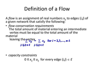
Step 0 [Initialization] Present a given LP problem in standard form and
set up initial tableau.
Step 1 [Optimality test] If all entries in the objective row are nonnegative —
stop: the tableau represents an optimal solution.
Step 2 [Find entering variable] Select (the most) negative entry in the
objective row. Mark its column to indicate the entering variable and the pivot column.
Step 3 [Find departing variable] For each positive entry in the pivot column, calculate the θ-ratio
by dividing that row's entry in the rightmost column by its entry in the pivot column. (If there are
no positive entries in the pivot column — stop: the problem is unbounded.) Find the row with the
smallest θ-ratio, mark this row to indicate the departing variable and the pivot row.
Step 4 [Form the next tableau] Divide all the entries in the pivot row by its entry in the pivot
column. Subtract from each of the other rows, including the objective row, the new pivot row
multiplied by the entry in the pivot column of the row in question. Replace the label of the pivot
row by the variable's name of the pivot column and go back to Step 1.](https://image.slidesharecdn.com/unit4-220307080125/85/Unit-4-13-320.jpg)
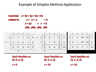
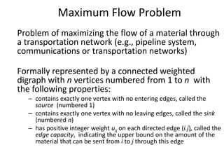
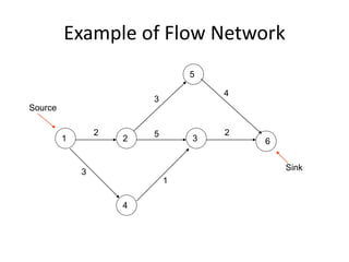

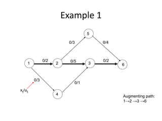
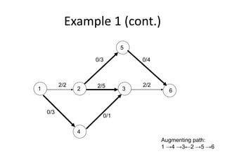
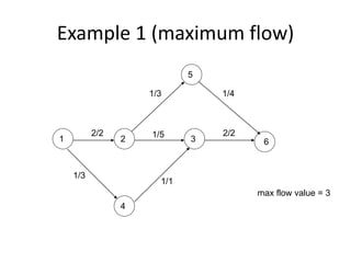
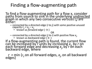
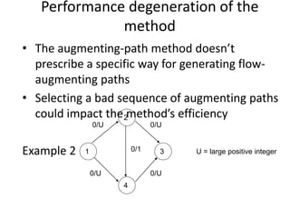
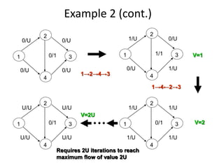
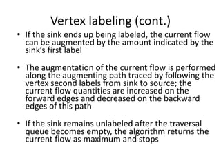
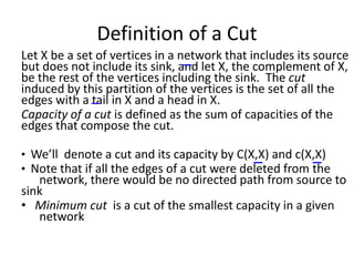
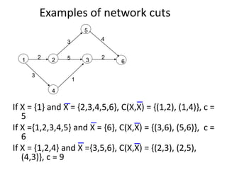

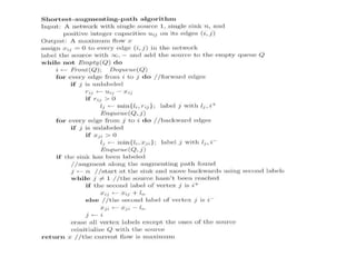
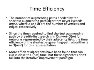


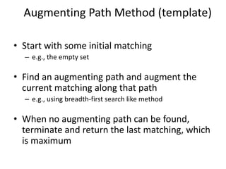

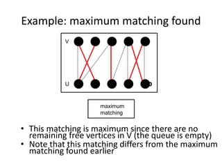


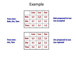
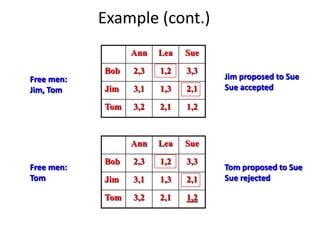


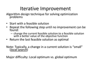
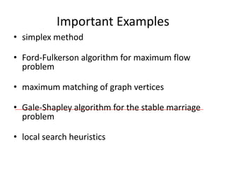
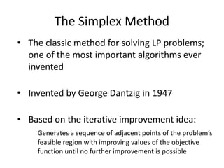
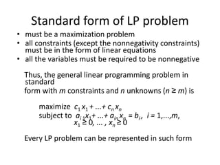
Iterative improvement is an algorithm design technique for solving optimization problems. It starts with a feasible solution and repeatedly makes small changes to the current solution to find a solution with a better objective function value until no further improvements can be found. The simplex method, Ford-Fulkerson algorithm, and local search heuristics are examples that use this technique. The maximum flow problem can be solved using the iterative Ford-Fulkerson algorithm, which finds augmenting paths in a flow network to incrementally increase the flow from the source to the sink until no more augmenting paths exist.