https://connpass.com/event/86005/

1. State Aware Imitation Learning
Y. Schroecker and C. L. Isbell
NIPS 2017
Eiji Uchibe

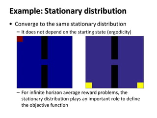
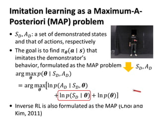
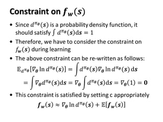
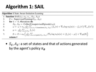
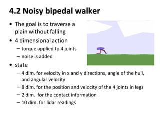
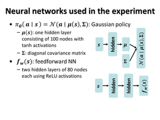
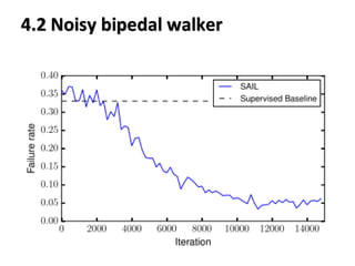
2. Why I choose this paper
• I was going to introduce “Learning Robust Rewards
with Adversarial Inverse Reinforcement Learning”
because it is closely related to my study
– This paper will be presented by Kobayashi-san
• So, I decided to talk about “State Aware Imitation
Learning”
– A stationary distribution is important in RL/IL, but it is not
carefully studied
– Our paper (Morimura et al., 2010) plays a critical role
– I’m trying to use it as a component of intrinsic motivation
to explore the environment efficiently

3. Notation
• 𝒔, 𝒂: (continuous) state and action
• 𝜋 𝜽(𝒂 ∣ 𝒔): stochastic policy parameterized by 𝜽
• 𝑝(𝒔′
∣ 𝒔, 𝒂): (unknown) state transition probability
• 𝑑 𝜋 𝜽 (𝒔): stationary distribution under 𝜋 𝜽
• 𝑝 𝜋 𝜽 𝒔′, 𝒂 𝒔 : forward transition probability related
to the forward Markov chain 𝑀(𝜽)
• 𝑞 𝜋 𝜽 𝒔, 𝒂 𝒔′
: backward transition probability
related to the backward Markov chain 𝐵(𝜽)

4. Example: Stationary distribution
• Consider the 9x9 grid world
• 5 actions (stop, left, right,
up, and down)
• Random policy
• Move to the intended
direction with probability0.9.
• Consider the limiting distribution
𝜋 𝒂 𝒔 = Τ1 5
𝑑 𝜋 𝒔 ≜ lim
𝑡→∞
Pr(𝑆𝑡 = 𝒔 ∣ 𝐴0:𝑡 ∼ 𝜋)

5. Example: Stationary distribution
• Converge to the same stationary distribution
– It does not depend on the starting state (ergodicity)
– For infinite horizon average reward problems, the
stationary distribution plays an important role to define
the objective function

6. Policy-Gradient theorem
• The objective function of the policy gradient RL
• Policy gradient algorithms provide a method to
evaluate 𝛻𝜽 𝐽(𝜽)
• Policy gradient theorem (Morimura et al., 2010)
– 𝑄 𝛾
𝜋 𝜽
, 𝑉𝛾
𝜋 𝜃
: value functions with discount factor 𝛾
𝛻𝜽 𝐽(𝜽) = ඵ𝑑 𝜋 𝜽 𝒔 𝜋 𝜽 𝒂 𝒔 𝛻𝜽 ln 𝜋 𝜽 𝒂 𝒔 𝑄 𝛾
𝜋 𝜽
𝒔, 𝒂 d𝒔d𝒂
𝐽 𝜽 = lim
𝑇→∞
1
𝑇
𝔼 𝑀 𝜽 ෍
𝑡=1
𝑇
𝑟𝑡 = ඵ𝑑 𝜋 𝜽 𝒔 𝜋 𝜽 𝒂 𝒔 𝑟 𝒔, 𝒂 d𝒔d𝒂
+(1 − 𝛾) න𝑑 𝜋 𝜽 𝒔 𝛻𝜽 ln 𝑑 𝜋 𝜽 𝒔 𝑉𝛾
𝜋 𝜽
𝒔 d𝒔

7. Policy-Gradient theorem
•
• The second term is usually ignored because 1 − 𝛾 ≈
0 in many settings
• We still need to samples from 𝑑 𝜋 𝜽 (𝒔) to evaluate the
policy gradient, but it is usually difficult
• 𝑑 𝜋 𝜽 (𝒔) is considered to derive algorithms, but a
different distribution is used in practice because
𝑑 𝜋 𝜽 (𝒔) is unknown and hard to estimate
𝛻𝜽 𝐽(𝜽) = ඵ𝑑 𝜋 𝜽 𝒔 𝜋 𝜽 𝒂 𝒔 𝛻𝜽 ln 𝜋 𝜽 𝒂 𝒔 𝑄 𝛾
𝜋 𝜽
𝒔, 𝒂 d𝒔d𝒂
+(1 − 𝛾) න𝑑 𝜋 𝜽 𝒔 𝛻𝜽 ln 𝑑 𝜋 𝜽 𝒔 𝑉𝛾
𝜋 𝜽
𝒔 d𝒔

8. Imitation learning as a Maximum-A-
Posteriori (MAP) problem
• 𝑆 𝐷, 𝐴 𝐷: a set of demonstrated states
and that of actions, respectively
• The goal is to find 𝜋 𝜽(𝒂 ∣ 𝒔) that
imitates the demonstrator’s
behavior, formulated as the MAP problem
• Inverse RL is also formulated as the MAP (Choi and
Kim, 2011)
arg max
𝜽
𝑝(𝜽 ∣ 𝑆 𝐷, 𝐴 𝐷)
+ln 𝑝(𝑆 𝐷 ∣ 𝜽) + ሿln 𝑝(𝜽)
= arg max
𝜽
ൣln 𝑝(𝐴 𝐷 ∣ 𝑆 𝐷, 𝜽)
𝑆 𝐷, 𝐴 𝐷

9. What is 𝒑(𝑺 𝑫 ∣ 𝜽)
•
• We can evaluate the first and the third terms easily
because 𝜋 𝜽(𝒂 ∣ 𝒔) is implemented by ourselves
• The role of ln 𝑝(𝑆 𝐷 ∣ 𝜽) is to reproduce states that
are similar to the ones in 𝑆 𝐷
• If it is not considered, the imitation policy has a
tendency to take actions that goes to states that are
not in 𝑆 𝐷 (Pomerleau, 1989; Ross and Bagnell, 2010)
arg max
𝜽
ln 𝑝(𝐴 𝐷 ∣ 𝑆 𝐷, 𝜽) + ln 𝑝(𝑆 𝐷 ∣ 𝜽) + ln 𝑝(𝜽)

10. State Aware Imitation Learning (SAIL)
• To solve the MAP problem, we need 𝛻𝜽 ln 𝑝(𝑆 𝐷 ∣ 𝜽)
• This paper assumes
• 𝜽 is updated by the following gradient
• The major contribution is to provide the estimator of
𝛻𝜽 𝑑 𝜋 𝜽(𝒔)
Δ𝜽 =
1
𝑆 𝐷
෍
𝒔,𝒂 ∈(𝑆 𝐷,𝐴 𝐷)
𝛻𝜽 ln 𝜋 𝜽(𝒂 ∣ 𝒔) + 𝛻𝜽 𝑑 𝜋 𝜽 𝑠 + 𝛻𝜽 𝑝(𝜽)
𝛻𝜃 ln 𝑝(𝐴 𝐷 ∣ 𝑆 𝐷, 𝜽) 𝛻𝜃 ln 𝑝(𝑆 𝐷 ∣ 𝜽)
𝛻𝜽 ln 𝑝 𝑆 𝐷 𝜽 = ෍
𝒔∈𝑆 𝐷
𝛻𝜽 ln 𝑑 𝜋 𝜽(𝒔)

11. 3.1 A temporal difference approach to …
• Definition of stationary distribution
• Because
we obtain the following relation
where
𝑑 𝜋 𝜽 𝒔′
= න𝑑 𝜋 𝜽 𝒔 𝜋 𝜽 𝒂 𝒔 𝑝 𝒔′
𝒔, 𝒂 d𝒔d𝒂
𝛻𝜽 𝑑 𝜋 𝜽 𝒔′
𝛻𝜽 𝑑 𝜋 𝜽 𝒔 𝜋 𝜽 𝒂 𝒔 𝑝 𝒔′
𝒔, 𝒂
= 𝑑 𝜋 𝜽 𝒔 𝜋 𝜽 𝒂 𝒔 𝑝 𝒔′
𝒔, 𝒂 𝛻𝜽 ln 𝑑 𝜋 𝜽 𝒔 + 𝛻𝜽 ln 𝜋 𝜽(𝒂 ∣ 𝒔)
= න𝑝 𝜋 𝜽 𝒔, 𝒂, 𝒔′ 𝛻𝜽 ln 𝑑 𝜋 𝜽 (𝒔) + 𝛻𝜽 ln 𝜋 𝜽 𝒂 𝒔 d𝒔d𝒂
𝑝 𝜋 𝜽 𝒔, 𝒂, 𝒔′
≜ 𝑑 𝜋 𝜽 𝒔 𝜋 𝜽 𝒂 𝒔 𝑝 𝒔′
𝒔, 𝒂

12. Reverse transition probability
• Dividing by 𝑑 𝜋 𝜽(𝒔′) yields
where
• 𝑞 𝜋 𝜽(𝒔, 𝒂 ∣ 𝒔′
) is called the backward Markov chain
while 𝑝 𝜋 𝜃(𝒔′, 𝒂 ∣ 𝒔) the forward Markov chain. See
Propositions 1 and 2 of Morimura et al. (2010) for
some theoretical properties
𝛻𝜽 ln 𝑑 𝜋 𝜽 𝒔′
= න𝑞 𝜋 𝜽 𝒔, 𝒂 ∣ 𝒔′ 𝛻𝜽 ln 𝑑 𝜋 𝜽(𝒔) + 𝛻𝜽 ln 𝜋 𝜽 𝒂 𝒔 d𝒔d𝒂
𝑞 𝜋 𝜽 𝒔, 𝒂 ∣ 𝒔′ ≜
𝑝 𝜋 𝜽 𝒔, 𝒂, 𝒔′
𝑑 𝜋 𝜽 𝒔′
reverse transition
probability

13. Temporal difference error
• Arranging the previous equation, the fundamental
equation to estimate 𝛻𝜽 ln 𝑑 𝜋 𝜽 (𝒔) can be obtained
where
– Note 𝜹 is a vector
• Recap: Temporal difference error of Q-learning
𝜹 𝒔, 𝒂, 𝒔′ ≜ 𝛻𝜽 ln 𝜋 𝜽 𝒂 𝒔 + 𝛻𝜽 ln 𝑑 𝜋 𝜽 𝒔
න𝑞 𝜋 𝜽 𝒔, 𝒂 𝒔′ 𝜹 𝒔, 𝒂, 𝒔′ d𝒔d𝒂 = 𝟎
−𝛻𝜽 ln 𝑑 𝜋 𝜽 𝒔′
𝛿 𝒔, 𝒂, 𝒔′ ≜ 𝑟 𝒔, 𝒂 + 𝛾 max
𝒂′
𝑄 𝒔′, 𝒂′ − 𝑄 𝒔, 𝒂

14. 3.2 Online temporal difference learning …
• This paper proposes an online TD learning algorithm,
which is suitable for deep neural networks
• 𝛻𝜽 ln 𝑑 𝜋 𝜽 (𝒔) is approximated by
– 𝒘: parameter of the approximator
– 𝒄: unknown constant vector
• Update rule
𝒇 𝒘 𝒔 ≈ 𝛻𝜽 ln 𝑑 𝜋 𝜽 𝒔 + 𝒄
Δ𝒘 = 𝛼𝛻𝒘 𝒇 𝒘 𝒔′ 𝛻𝜽 ln 𝜋 𝜽(𝒂 ∣ 𝒔) +𝒇 𝒘 𝒔 − 𝒇 𝒘 𝒔′
TD error
target valuegradient
(matrix?)

15. Constraint on 𝒇 𝒘(𝒔)
• Since 𝑑 𝜋 𝜽(𝒔) is a probabilitydensity function, it
should satisfy ∫ 𝑑 𝜋 𝜽 𝒔 d𝒔 = 1
• Therefore, we have to consider the constraint on
𝑓𝒘(𝒔) during learning
• The above constraint can be re-written as follows:
• This constraint is satisfied by setting c appropriately
𝔼 𝑑 𝜋 𝜽 𝛻𝜽 ln 𝑑 𝜋 𝜽 𝒔 = න𝑑 𝜋 𝜽 𝒔 𝛻𝜽 ln 𝑑 𝜋 𝜽(𝒔)d𝒔
= න𝛻𝜽 𝑑 𝜋 𝜽(𝒔)d𝒔 = 𝛻𝜽 න𝑑 𝜋 𝜽 𝒔 d𝒔 = 𝛻𝜽 1 = 𝟎
𝒇 𝒘 𝒔 ≈ 𝛻𝜽 ln 𝑑 𝜋 𝜽 𝒔 + 𝔼 𝒇 𝒘 𝒔

16. Algorithm 1: SAIL
• 𝑆 𝐸, 𝐴 𝐸: a set of states and that of actions generated
by the agent’s policy 𝜋 𝜽

17. 4.2 Noisy bipedal walker
• The goal is to traverse a
plain without falling
• 4 dimensional action
– torque applied to 4 joints
– noise is added
• state
– 4 dim. for velocity in x and y directions, angle of the hull,
and angular velocity
– 8 dim. for the position and velocity of the 4 joints in legs
– 2 dim. for the contact information
– 10 dim. for lidar readings

18. Neural networks used in the experiment
• 𝜋 𝜽 𝒂 𝒔 = 𝒩(𝒂 ∣ 𝝁 𝒔 , 𝚺): Gaussian policy
– 𝝁(𝒔): one hidden layer
consisting of 100 nodes with
tanh activations
– 𝚺: diagonal covariance matrix
• 𝒇 𝒘(𝒔): feedforward NN
– two hidden layers of 80 nodes
each using ReLU activations
𝒔 𝝁
hidden
𝚺
𝒩(𝒂∣𝝁𝒔,𝚺)
𝒔
hidden
hidden
𝒇𝒘(𝒔)

19. 4.2 Noisy bipedal walker

20. My opinions
• Is learning the gradient of 𝑑 𝜋 𝜃 easier than learning a
value function?
• The dimension of the gradient is equal to the number
of parameters of the policy. In general, it is too huge
if we use a deep NN policy
• The technique of the target network is not used
• Trust region framework should be introduced to
avoid catastrophic changes

21. References
• Choi, J. and Kim, K.-E. (2011). Map inference for Bayesian inverse
reinforcement learning. NIPS 24.
• Morimura, T. Uchibe, E., Yoshimoto, J., Peters, J., and Doya, K. (2010).
Derivatives of Logarithmic Stationary Distributions for Policy Gradient
Reinforcement Learning. Neural Computation, 22, 342-376.
• Pomerleau, D. A. (1989). ALVINN: An autonomous land vehicle in a neural
network. NIPS 1.
• Ross, S., and Bagnell, J. A. (2010). Efficient Reductions for Imitation
Learning. In Proc. of 13th AISTATS.
• Schroecker, Y., and Isbell, C. L. (2017). State Aware Imitation Learning.
NIPS 30.