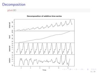
Downloaded 23 times
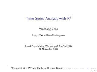

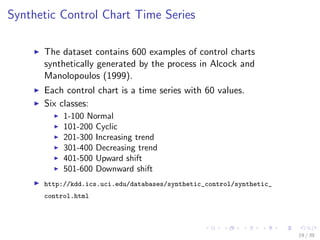
![Time Series Data in R
a <- ts(1:20, frequency = 12, start = c(2011, 3))
print(a)
## Jan Feb Mar Apr May Jun Jul Aug Sep Oct Nov Dec
## 2011 1 2 3 4 5 6 7 8 9 10
## 2012 11 12 13 14 15 16 17 18 19 20
str(a)
## Time-Series [1:20] from 2011 to 2013: 1 2 3 4 5 6 7 8 9 10...
attributes(a)
## $tsp
## [1] 2011 2013 12
##
## $class
## [1] "ts"
6 / 39](https://image.slidesharecdn.com/rdatamining-slides-time-series-analysis-160711201918/85/R-data-mining-Time-Series-Analysis-with-R-6-320.jpg)
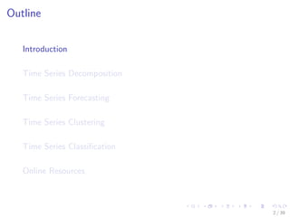
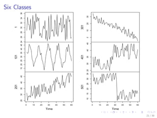
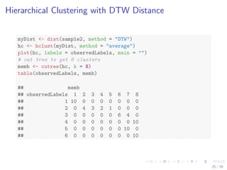
![Synthetic Control Chart Time Series
# read data into R sep='': the separator is white space, i.e., one
# or more spaces, tabs, newlines or carriage returns
sc <- read.table("./data/synthetic_control.data", header = F, sep = "")
# show one sample from each class
idx <- c(1, 101, 201, 301, 401, 501)
sample1 <- t(sc[idx, ])
plot.ts(sample1, main = "")
20 / 39](https://image.slidesharecdn.com/rdatamining-slides-time-series-analysis-160711201918/85/R-data-mining-Time-Series-Analysis-with-R-20-320.jpg)
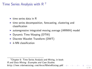
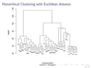
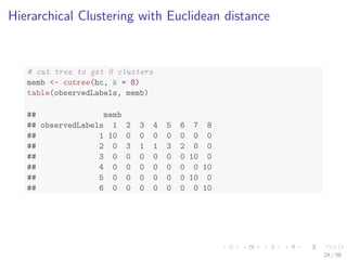
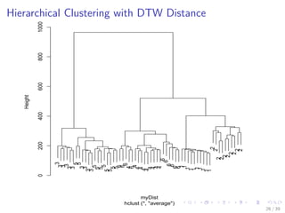
![Hierarchical Clustering with Euclidean distance
# sample n cases from every class
n <- 10
s <- sample(1:100, n)
idx <- c(s, 100 + s, 200 + s, 300 + s, 400 + s, 500 + s)
sample2 <- sc[idx, ]
observedLabels <- rep(1:6, each = n)
# hierarchical clustering with Euclidean distance
hc <- hclust(dist(sample2), method = "ave")
plot(hc, labels = observedLabels, main = "")
22 / 39](https://image.slidesharecdn.com/rdatamining-slides-time-series-analysis-160711201918/85/R-data-mining-Time-Series-Analysis-with-R-22-320.jpg)
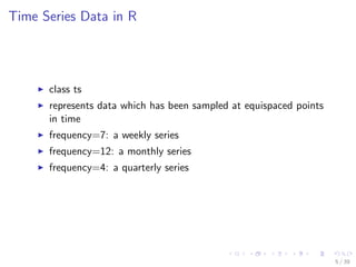
![Decision Tree
pClassId <- predict(ct)
table(classId, pClassId)
## pClassId
## classId 1 2 3 4 5 6
## 1 100 0 0 0 0 0
## 2 1 97 2 0 0 0
## 3 0 0 99 0 1 0
## 4 0 0 0 100 0 0
## 5 4 0 8 0 88 0
## 6 0 3 0 90 0 7
# accuracy
(sum(classId == pClassId))/nrow(sc)
## [1] 0.8183
30 / 39](https://image.slidesharecdn.com/rdatamining-slides-time-series-analysis-160711201918/85/R-data-mining-Time-Series-Analysis-with-R-30-320.jpg)
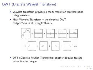
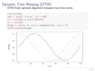
![DWT (Discrete Wavelet Transform)
# extract DWT (with Haar filter) coefficients
library(wavelets)
wtData <- NULL
for (i in 1:nrow(sc)) {
a <- t(sc[i, ])
wt <- dwt(a, filter = "haar", boundary = "periodic")
wtData <- rbind(wtData, unlist(c(wt@W, wt@V[[wt@level]])))
}
wtData <- as.data.frame(wtData)
wtSc <- data.frame(cbind(classId, wtData))
32 / 39](https://image.slidesharecdn.com/rdatamining-slides-time-series-analysis-160711201918/85/R-data-mining-Time-Series-Analysis-with-R-32-320.jpg)
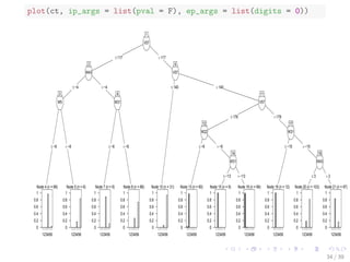
![Decision Tree with DWT
ct <- ctree(classId ~ ., data = wtSc,
controls = ctree_control(minsplit=20, minbucket=5,
maxdepth=5))
pClassId <- predict(ct)
table(classId, pClassId)
## pClassId
## classId 1 2 3 4 5 6
## 1 98 2 0 0 0 0
## 2 1 99 0 0 0 0
## 3 0 0 81 0 19 0
## 4 0 0 0 74 0 26
## 5 0 0 16 0 84 0
## 6 0 0 0 3 0 97
(sum(classId==pClassId)) / nrow(wtSc)
## [1] 0.8883
33 / 39](https://image.slidesharecdn.com/rdatamining-slides-time-series-analysis-160711201918/85/R-data-mining-Time-Series-Analysis-with-R-33-320.jpg)
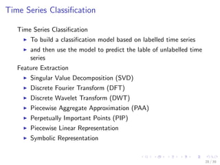
![k-NN Classification
find the k nearest neighbours of a new instance
label it by majority voting
needs an efficient indexing structure for large datasets
k <- 20
newTS <- sc[501, ] + runif(100) * 15
distances <- dist(newTS, sc, method = "DTW")
s <- sort(as.vector(distances), index.return = TRUE)
# class IDs of k nearest neighbours
table(classId[s$ix[1:k]])
##
## 4 6
## 3 17
35 / 39](https://image.slidesharecdn.com/rdatamining-slides-time-series-analysis-160711201918/85/R-data-mining-Time-Series-Analysis-with-R-35-320.jpg)
![k-NN Classification
find the k nearest neighbours of a new instance
label it by majority voting
needs an efficient indexing structure for large datasets
k <- 20
newTS <- sc[501, ] + runif(100) * 15
distances <- dist(newTS, sc, method = "DTW")
s <- sort(as.vector(distances), index.return = TRUE)
# class IDs of k nearest neighbours
table(classId[s$ix[1:k]])
##
## 4 6
## 3 17
Results of majority voting: class 6
35 / 39](https://image.slidesharecdn.com/rdatamining-slides-time-series-analysis-160711201918/85/R-data-mining-Time-Series-Analysis-with-R-36-320.jpg)

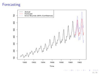
The document discusses time series analysis techniques in R, including decomposition, forecasting, clustering, and classification. It provides an overview of methods such as ARIMA modeling, dynamic time warping, discrete wavelet transforms, and decision trees. Examples are shown applying these techniques to air passenger data and synthetic control chart time series data, including decomposing, forecasting, hierarchical clustering with Euclidean and DTW distances, and classifying with decision trees using DWT features. Accuracy of over 80% is achieved on the classification tasks.


![[DSC Europe 25] Ivan Lukovic & Marija Djukic - From Data to Value: Why Maturi...](https://cdn.slidesharecdn.com/ss_thumbnails/ahrfps8xr6knowwhacxh-1-ivan-marija-dsc-2025-ld-v1-presentation-260115093812-be21adfc-thumbnail.jpg?width=640&height=640&fit=bounds)


![[DSC Europe 25] Andrzej Kowalczyk - AI - how to start small and grow in the f...](https://cdn.slidesharecdn.com/ss_thumbnails/oy1zmo94qv6vpcqjvno2-andrzej-kowalczyk-ai-how-to-start-small-and-grow-in-the-future-1-260119121559-cf093b23-thumbnail.jpg?width=640&height=640&fit=bounds)
