Downloaded 16 times


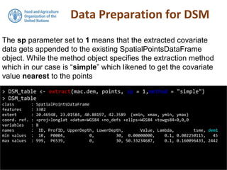
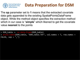
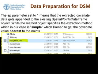
![Coordinates
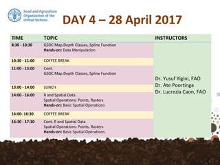
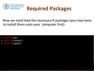
> coordinates(pointdata) <- ~X + Y
> str(pointdata)
Formal class 'SpatialPointsDataFrame' [package "sp"] with 5 slots
..@ data :'data.frame': 3302 obs. of 7 variables:
.. ..$ ID : int [1:3302] 4 7 8 9 10 11 12 13 14 15 ...
.. ..$ ProfID : Factor w/ 3228 levels "P0004","P0007",..: 1 2 3 4
5 6 7 8 9 10 ...
.. ..$ UpperDepth: int [1:3302] 0 0 0 0 0 0 0 0 0 0 ...
.. ..$ LowerDepth: int [1:3302] 30 30 30 30 30 30 30 30 30 30 ...
.. ..$ Value : num [1:3302] 11.88 3.49 2.32 1.94 1.34 ...
.. ..$ Lambda : num [1:3302] 0.1 0.1 0.1 0.1 0.1 0.1 0.1 0.1 0.1
0.1 ...
.. ..$ tsme : num [1:3302] 0.1601 0.00257 0.0026 0.00284 0.00268
...
..@ coords.nrs : int [1:2] 3 4
..@ coords : num [1:3302, 1:2] 7485085 7486492 7485564 7495075
7494798 ...
.. ..- attr(*, "dimnames")=List of 2
.. .. ..$ : chr [1:3302] "1" "2" "3" "4" ...
.. .. ..$ : chr [1:2] "X" "Y"
..@ bbox : num [1:2, 1:2] 7455723 4526565 7667660 4691342
.. ..- attr(*, "dimnames")=List of 2
.. .. ..$ : chr [1:2] "X" "Y"
.. .. ..$ : chr [1:2] "min" "max"](https://image.slidesharecdn.com/d4-2-getting-spatial-170531132033/85/10-Getting-Spatial-9-320.jpg)
![Coordinates
> coordinates(pointdata) <- ~X + Y
> str(pointdata)
Formal class 'SpatialPointsDataFrame' [package "sp"] with 5 slots
..@ data :'data.frame': 3302 obs. of 7 variables:
.. ..$ ID : int [1:3302] 4 7 8 9 10 11 12 13 14 15 ...
.. ..$ ProfID : Factor w/ 3228 levels "P0004","P0007",..: 1 2 3 4
5 6 7 8 9 10 ...
.. ..$ UpperDepth: int [1:3302] 0 0 0 0 0 0 0 0 0 0 ...
.. ..$ LowerDepth: int [1:3302] 30 30 30 30 30 30 30 30 30 30 ...
.. ..$ Value : num [1:3302] 11.88 3.49 2.32 1.94 1.34 ...
.. ..$ Lambda : num [1:3302] 0.1 0.1 0.1 0.1 0.1 0.1 0.1 0.1 0.1
0.1 ...
.. ..$ tsme : num [1:3302] 0.1601 0.00257 0.0026 0.00284 0.00268
...
..@ coords.nrs : int [1:2] 3 4
..@ coords : num [1:3302, 1:2] 7485085 7486492 7485564 7495075
7494798 ...
.. ..- attr(*, "dimnames")=List of 2
.. .. ..$ : chr [1:3302] "1" "2" "3" "4" ...
.. .. ..$ : chr [1:2] "X" "Y"
..@ bbox : num [1:2, 1:2] 7455723 4526565 7667660 4691342
.. ..- attr(*, "dimnames")=List of 2
.. .. ..$ : chr [1:2] "X" "Y"
.. .. ..$ : chr [1:2] "min" "max"
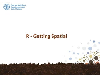
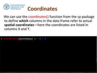
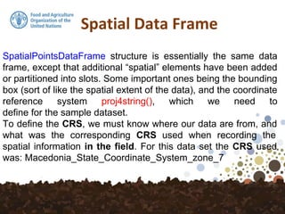
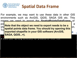
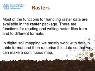
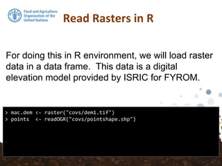
Note that by using the str function, the class
of pointdata has now changed from a
dataframe to a SpatialPointsDataFrame.
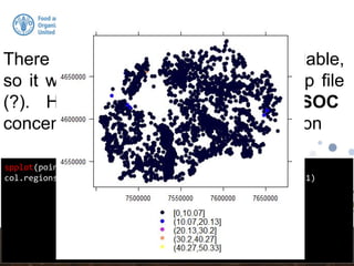
We can do a spatial plot of these points
using the spplot plotting function in the sp
package.](https://image.slidesharecdn.com/d4-2-getting-spatial-170531132033/85/10-Getting-Spatial-10-320.jpg)
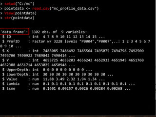
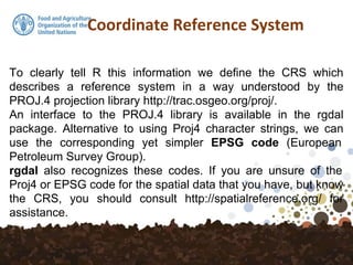
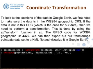


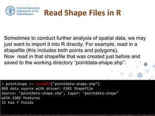
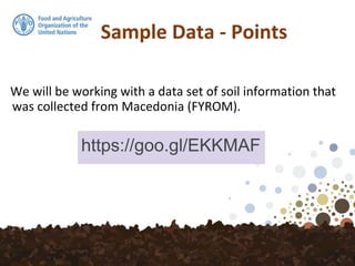
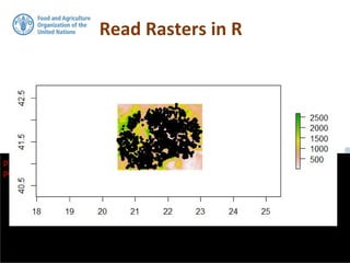
![The imported shapefile is now a SpatialPointsDataFrame, just
like the pointdata data that was worked on before, and is
ready for further analysis.
Read Shape Files in R
> str(pointshape)
Formal class 'SpatialPointsDataFrame' [package "sp"] with 5 slots
..@ data :'data.frame': 3302 obs. of 7 variables:
...](https://image.slidesharecdn.com/d4-2-getting-spatial-170531132033/85/10-Getting-Spatial-25-320.jpg)
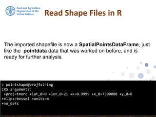
![The imported shapefile is now a SpatialPointsDataFrame, just
like the pointdata data that was worked on before, and is
ready for further analysis.
Read Shape Files in R
> str(pointshape)
Formal class 'SpatialPointsDataFrame' [package "sp"] with 5 slots
..@ data :'data.frame': 3302 obs. of 7 variables:
...](https://image.slidesharecdn.com/d4-2-getting-spatial-170531132033/85/10-Getting-Spatial-26-320.jpg)
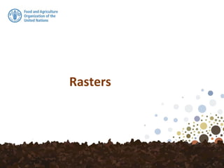
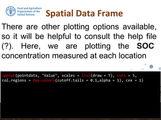
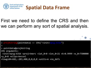
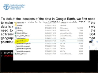
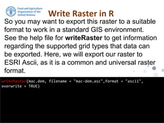
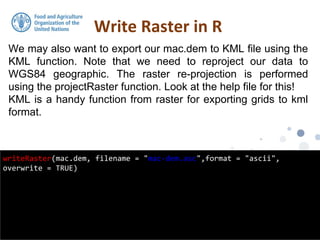
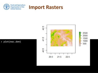
![For doing this in R environment, we will load raster
data in a data frame. This data is a digital
elevation model provided by ISRIC for FYROM.
Read Rasters in R
> str(mac.dem)
Formal class 'RasterLayer' [package "raster"] with 12 slots
..@ file :Formal class '.RasterFile' [package "raster"] with 13
slots
.. .. ..@ name : chr "C:mccovsdem1.tif"
.. .. ..@ datanotation: chr "INT2S"
.. .. ..@ byteorder : chr "little"
.. .. ..@ nodatavalue : num -Inf
.. .. ..@ NAchanged : logi FALSE
.. .. ..@ nbands : int 1](https://image.slidesharecdn.com/d4-2-getting-spatial-170531132033/85/10-Getting-Spatial-31-320.jpg)


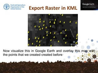
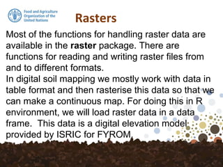
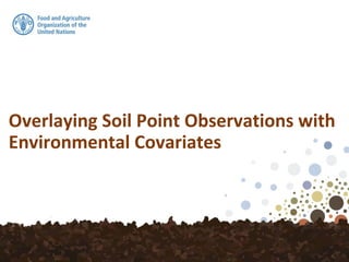
![The imported raster read.grid is a SpatialGridDataFrame,
which is a class of the sp package. To be able to use the raster
functions from raster we need to convert it to the RasterLayer
class.
Import Rasters
> str(grid.dem)
Formal class 'RasterLayer' [package "raster"] with 12 slots
..@ file :Formal class '.RasterFile' [package "raster"] with 13
slots
.. .. ..@ name : chr ""
.. .. ..@ datanotation: chr "FLT4S"
.. .. ..@ byteorder : chr "little"
.. .. ..@ nodatavalue : num -Inf
.. .. ..@ NAchanged : logi FALSE
.. .. ..@ nbands : int 1
.. .. ..@ bandorder : chr "BIL"
.. .. ..@ offset : int 0
.. .. ..@ toptobottom : logi TRUE
.. .. ..@ blockrows : int 0](https://image.slidesharecdn.com/d4-2-getting-spatial-170531132033/85/10-Getting-Spatial-41-320.jpg)

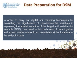

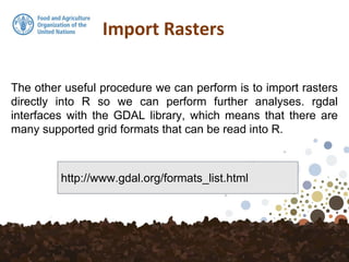
![Using Covariates from Disc
> list.files(path = "C:/mc/covs", pattern = ".tif$",
+ full.names = TRUE)
[1] "C:/mc/covs/dem.tif" "C:/mc/covs/dem1.tif" "C:/mc/covs/prec.tif"
"C:/mc/covs/slp.tif"
> list.files(path = "C:/mc/covs")
[1] "dem.tif" "dem1.tfw" "dem1.tif"
"dem1.tif.aux.xml" "dem1.tif.ovr"
[6] "desktop.ini" "pointshape.cpg" "pointshape.dbf"
"pointshape.prj" "pointshape.sbn"
[11] "pointshape.sbx" "pointshape.shp" "pointshape.shx"
"prec.tif" "slp.tif"
This utility is obviously a very handy feature when we are
working with large or large number of rasters. The work function
we need is list.files. For example:](https://image.slidesharecdn.com/d4-2-getting-spatial-170531132033/85/10-Getting-Spatial-51-320.jpg)
![Using Covariates from Disc
> list.files(path = "C:/mc/covs", pattern = ".tif$",
+ full.names = TRUE)
[1] "C:/mc/covs/dem.tif" "C:/mc/covs/dem1.tif" "C:/mc/covs/prec.tif"
"C:/mc/covs/slp.tif"
> list.files(path = "C:/mc/covs")
[1] "dem.tif" "dem1.tfw" "dem1.tif"
"dem1.tif.aux.xml" "dem1.tif.ovr"
[6] "desktop.ini" "pointshape.cpg" "pointshape.dbf"
"pointshape.prj" "pointshape.sbn"
[11] "pointshape.sbx" "pointshape.shp" "pointshape.shx"
"prec.tif" "slp.tif"
This utility is obviously a very handy feature when we are
working with large or large number of rasters. The work function
we need is list.files. For example:](https://image.slidesharecdn.com/d4-2-getting-spatial-170531132033/85/10-Getting-Spatial-52-320.jpg)
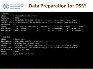
![Using Covariates from Disc
Covs <- list.files(path = "C:/mc/covs", pattern = ".tif$",full.names
= TRUE)
> Covs
[1] "C:/mc/covs/dem.tif" "C:/mc/covs/dem1.tif" "C:/mc/covs/prec.tif"
"C:/mc/covs/slp.tif"
> covStack <- stack(Covs)
> covStack
Error in compareRaster(rasters) : different extent
When the covariates in common resolution and extent, rather
than working with each raster independently it is more efficient to
stack them all into a single object. The stack function from raster
is ready-made for this, and is
simple as follow,](https://image.slidesharecdn.com/d4-2-getting-spatial-170531132033/85/10-Getting-Spatial-53-320.jpg)
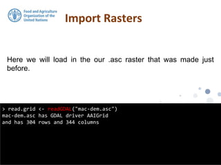
![Using Covariates from Disc
Covs <- list.files(path = "C:/mc/covs", pattern = ".tif$",full.names
= TRUE)
> Covs
[1] "C:/mc/covs/dem.tif" "C:/mc/covs/dem1.tif" "C:/mc/covs/prec.tif"
"C:/mc/covs/slp.tif"
> covStack <- stack(Covs)
> covStack
Error in compareRaster(rasters) : different extent
If the rasters are not in same resolution and extent you will find
the other raster package functions resample and projectRaster as
invaluable methods for harmonizing all your different raster layers.](https://image.slidesharecdn.com/d4-2-getting-spatial-170531132033/85/10-Getting-Spatial-54-320.jpg)

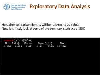
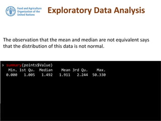
![Exploratory Data Analysis
We will continue using the DSM_table object that we created in the
previous section. As the data set was saved to file you will also find it
in your working directory.
> str(points)
Formal class 'SpatialPointsDataFrame' [package "sp"] with 5 slots
..@ data :'data.frame': 3302 obs. of 7 variables:
.. ..$ ID : Factor w/ 3228 levels "10","100","1000",..: 1896
3083 3136 3172 1 66 117 141 144 179 ...
.. ..$ ProfID : Factor w/ 3228 levels "P0004","P0007",..: 1 2 3 4
5 6 7 8 9 10 ...
.. ..$ UpperDepth: Factor w/ 1 level "0": 1 1 1 1 1 1 1 1 1 1 ...
.. ..$ LowerDepth: Factor w/ 1 level "30": 1 1 1 1 1 1 1 1 1 1 ...
.. ..$ Value : num [1:3302] 11.88 3.49 2.32 1.94 1.34 ...
.. ..$ Lambda : num [1:3302] 0.1 0.1 0.1 0.1 0.1 0.1 0.1 0.1 0.1
0.1 ...](https://image.slidesharecdn.com/d4-2-getting-spatial-170531132033/85/10-Getting-Spatial-56-320.jpg)


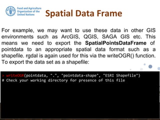
This document summarizes steps for working with spatial point data in R, including: 1. Importing point data from a CSV file and defining the coordinate columns; 2. Specifying the coordinate reference system of the data; 3. Plotting the data spatially and exporting to common GIS formats like shapefiles; 4. Transforming the data to a different CRS (WGS84) in order to visualize in Google Earth.


![Spatial_Data_Analysis_with_open_source_softwares[1]](https://cdn.slidesharecdn.com/ss_thumbnails/8db4d971-8e8c-4fd8-8682-b20e5d6cd65f-161221072847-thumbnail.jpg?width=640&height=640&fit=bounds)


