Download to read offline

![Matrix
y <- matrix(nrow=2,ncol=2)
y[1,1] <- 1
y[2,1] <- 2
y[1,2] <- 3
y[2,2] <- 4
x <- matrix(1:4, 2, 2)
A matrix is a vector
with two additional
attributes: the
number of rows and
the
number of columns
Matrix Operations
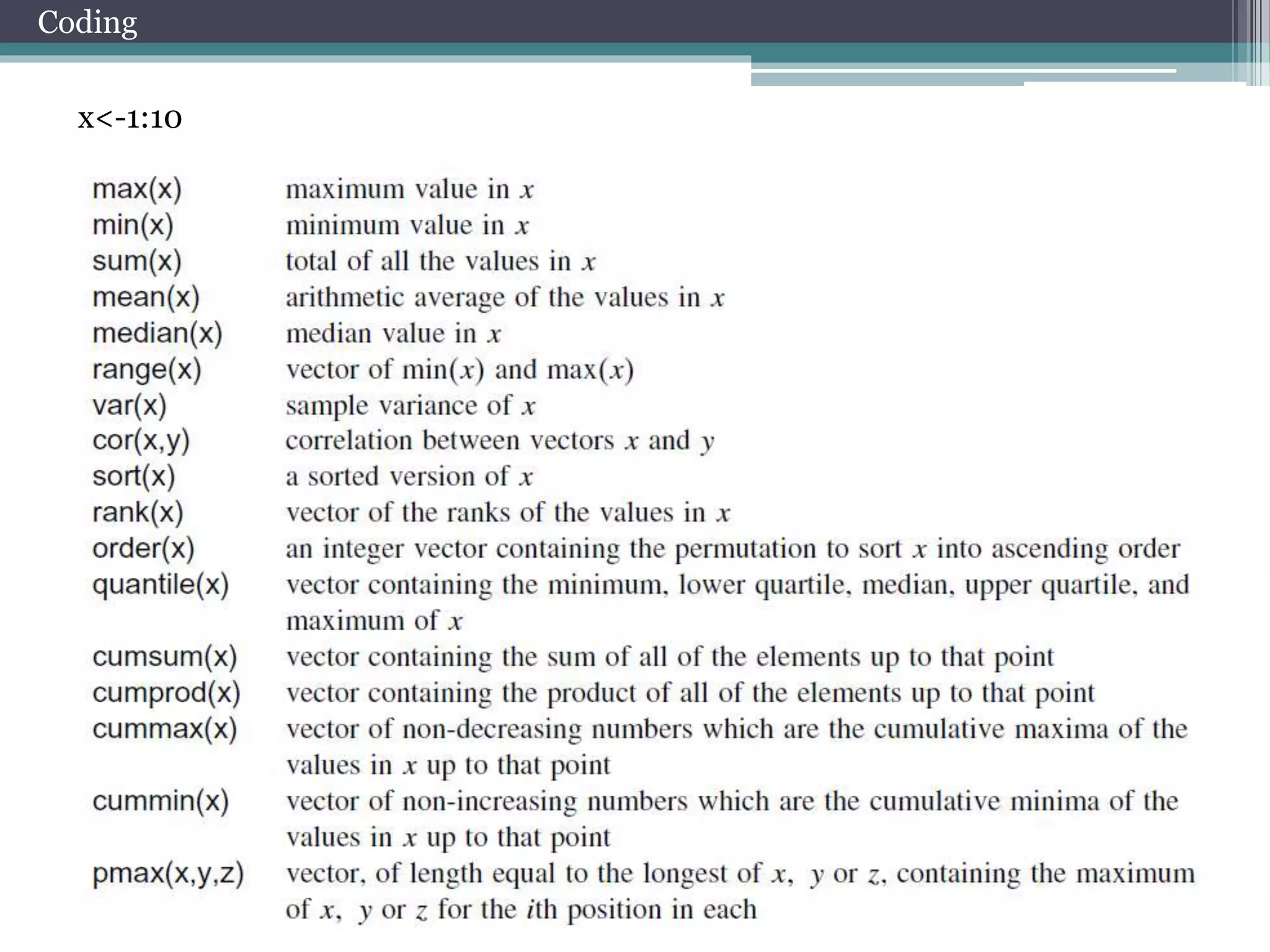
Coding
x %*% y
x* y
3*y
x+y
x+3
x[,2]
x[1,]
rbind(x,y)->z
cbind(x,y)
z[1:2,]
z[z[,1]>1,]
z[which(z[,1]>1),1]](https://image.slidesharecdn.com/seminarpsu10-141008013342-conversion-gate02/75/Seminar-PSU-10-10-2014-mme-7-2048.jpg)
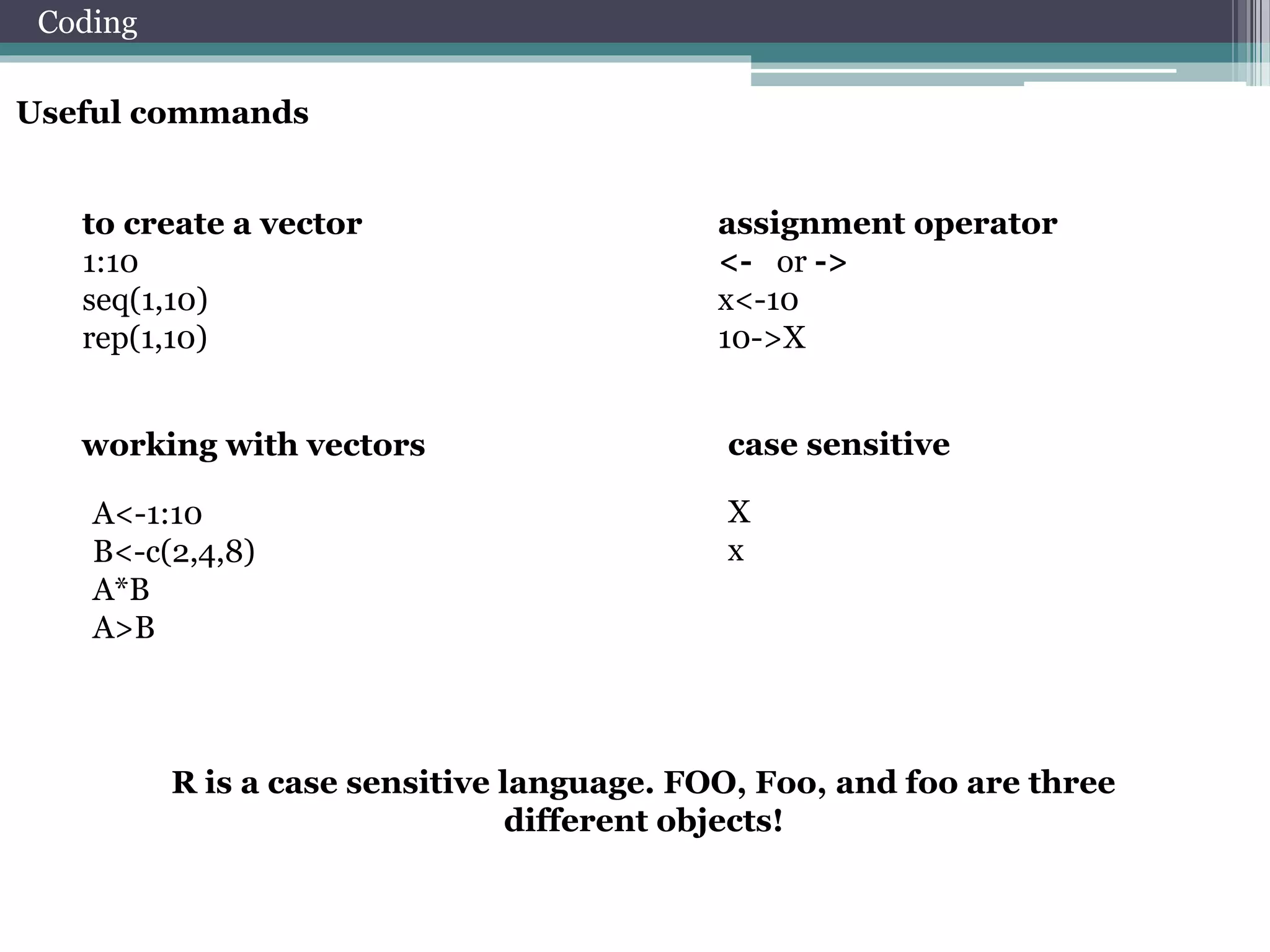
![List
j <- list(name="Joe", salary=55000, union=T)
j$salary
j[["salary"]]
j[[2]]
j$name [2]<-”Poll”
j$salary[2]<-10000
j$union [2]<-”F”
In contrast to a
vector, in which all
elements
must be of the same
mode, R’s list
structure can
combine objects of
different
types.
Data Frame
Coding
kids <- c("Jack","Jill")
ages <- c(12,10)
d <- data.frame(kids,ages)
d[1,]
d[,1]
d[[1]]
Arrays
my.array <- array(1:24, dim=c(3,4,2))
a data frame is like a
matrix, with a two-dimensional rows-andcolumns
structure. However, it differs from
a matrix in that each column may have a
different
mode.](https://image.slidesharecdn.com/seminarpsu10-141008013342-conversion-gate02/75/Seminar-PSU-10-10-2014-mme-8-2048.jpg)
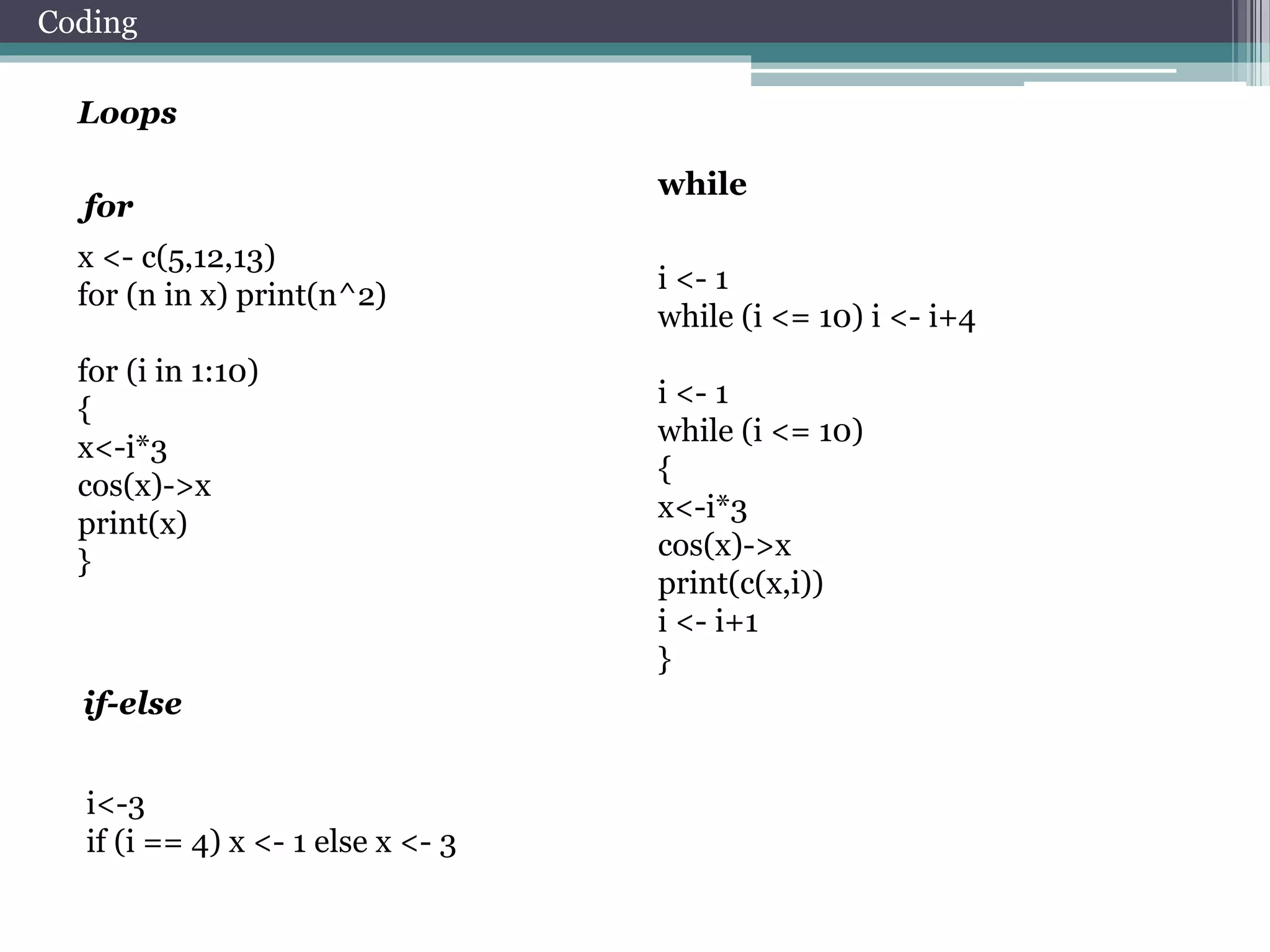

![Select data from matrix
x <- matrix(0,50,2)
x[,1]
x[1,]
x[,1]<-rnorm(50)
x
x[1,]<-rnorm(2)
x
x <- matrix(rnorm(100),50,2)
x[which(x[,1]>0),]
Operators
and &
or |](https://image.slidesharecdn.com/seminarpsu10-141008013342-conversion-gate02/75/Seminar-PSU-10-10-2014-mme-13-2048.jpg)
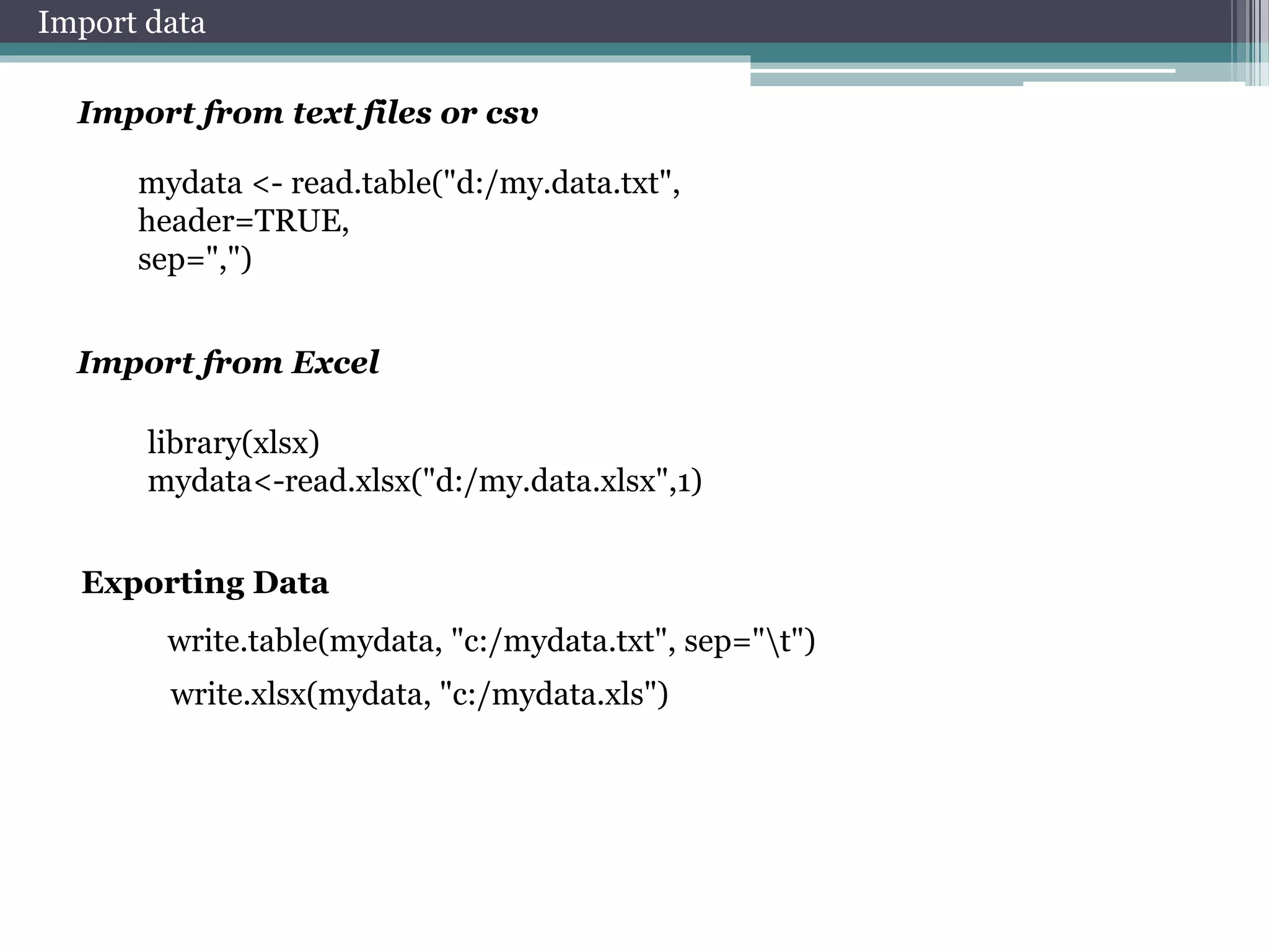
![Estimation of parameters
Let’s estimate parameters of
chosen distribution….
library(MASS)
fitdistr(x,"normal")
params<-fitdistr(x,"normal")$estimate
Compare theoretical and empirical
distributions…
hist(x, freq = FALSE,ylim=c(0,0.4))
curve(dnorm(x, params[1], params[2]), col = 2, add = TRUE)](https://image.slidesharecdn.com/seminarpsu10-141008013342-conversion-gate02/75/Seminar-PSU-10-10-2014-mme-17-2048.jpg)
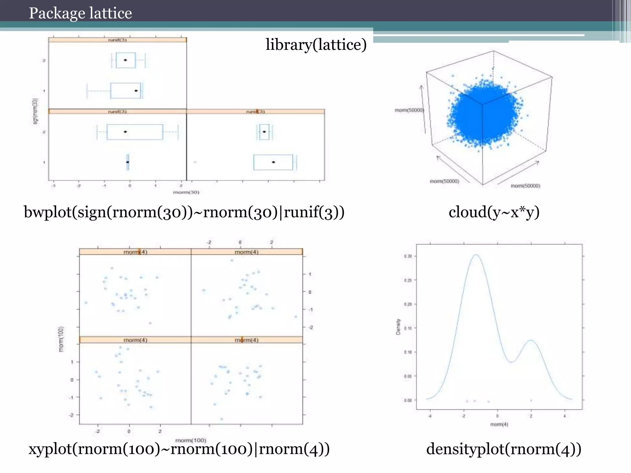
![Working with package quantmod
Data visualization
barChart(AAPL)
candleChart(AAPL,multi.col=TRUE,theme="white")
chartSeries(AAPL,up.col='white',dn.col='blue')
Add technical indicators
addMACD()
addBBands()
Data management
to.weekly(AAPL)
to.monthly(AAPL)
dailyReturn(AAPL)
weeklyReturn(AAPL)
monthlyReturn(AAPL)
Select data
AAPL['2007']
AAPL['2007-03/2007']
AAPL['/2007']
AAPL['2007-01-03']](https://image.slidesharecdn.com/seminarpsu10-141008013342-conversion-gate02/75/Seminar-PSU-10-10-2014-mme-25-2048.jpg)

![Practice № 1. Working with data
1. AFLT
2. GAZP
3. RTKM
4. ROSN
5. SBER
6. SBERP
7. HYDR
8. LKOH
9. VTBR
10. GMKN
11. SIBN
12. PLZL
13. MTSS
14. CHMF
15. SNGS
TASK:
a. Download Data of your instrument
b. Plot price
c. Add technical indicators
d. Calculate price returns
Commands to help :
barChart(AAPL)
chartSeries(AAPL,up.col='white',dn.col='blue')
AAPL['2007-03/2007']
addMACD()
dailyReturn(AAPL)](https://image.slidesharecdn.com/seminarpsu10-141008013342-conversion-gate02/75/Seminar-PSU-10-10-2014-mme-27-2048.jpg)
![Practice № 2. Distribution of price returns
1. AFLT
2. GAZP
3. RTKM
4. ROSN
5. SBER
6. SBERP
7. HYDR
8. LKOH
9. VTBR
10. GMKN
11. SIBN
12. PLZL
13. MTSS
14. CHMF
15. SNGS
TASK :
a. Download Data of your instrument
b. Calculate returns of close prices
c. Plot density of distribution
d. Estimate parameters of distribution
e. Plot in one graph empirical and theoretical
distributions
Commands to help :
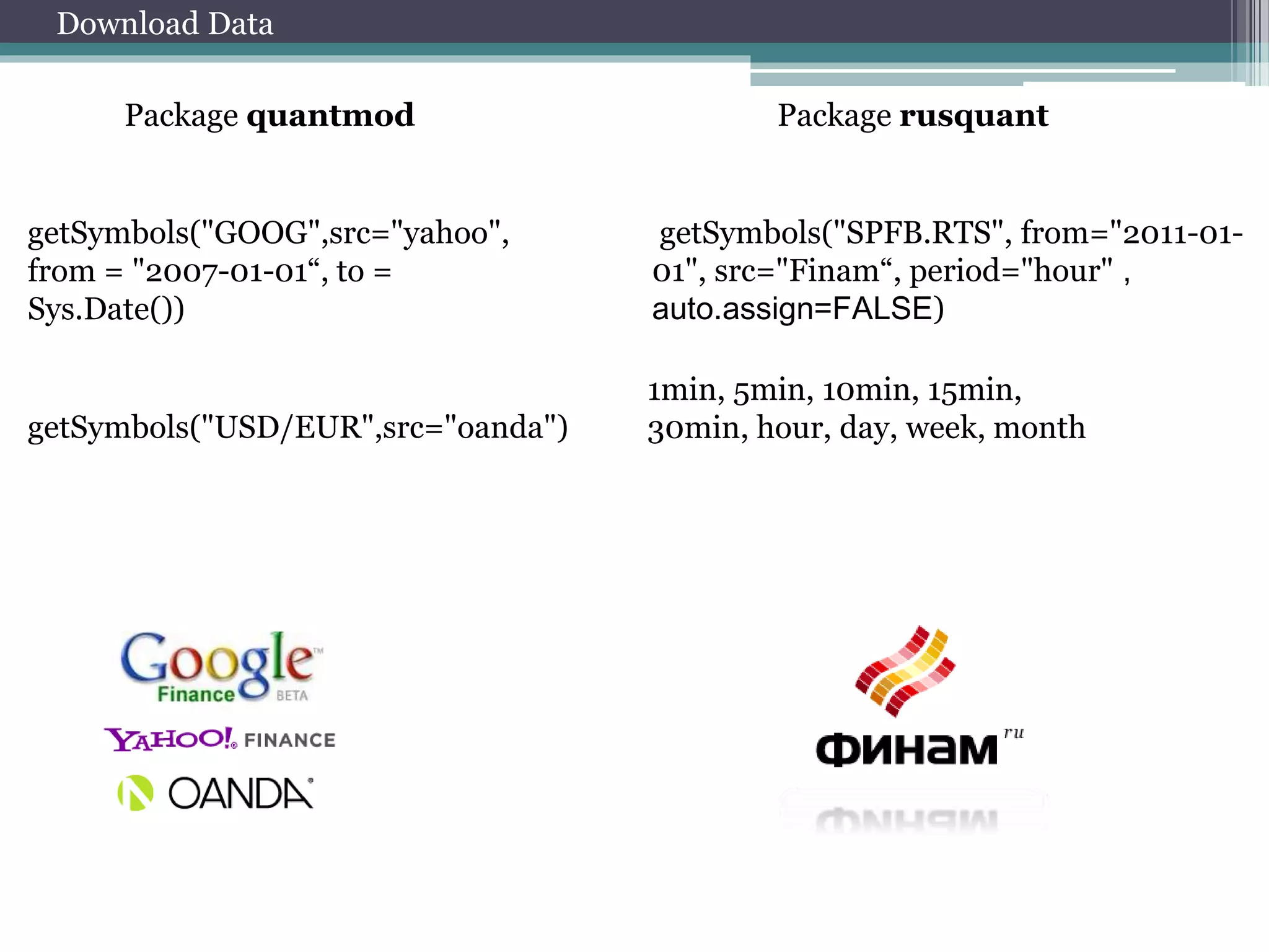
getSymbols("AFLT",
src="Finam", period="day" , auto.assign=FALSE)
library(MASS)
fitdistr(x,"normal")
hist(x)
density(x)
curve(dnorm(x, params[1], params[2]), col = 2, add = TRUE)](https://image.slidesharecdn.com/seminarpsu10-141008013342-conversion-gate02/75/Seminar-PSU-10-10-2014-mme-28-2048.jpg)
![Practice № 3. Estimation of correlation
1. AFLT
2. GAZP
3. RTKM
4. ROSN
5. SBER
6. SBERP
7. HYDR
8. LKOH
9. VTBR
10. GMKN
11. SIBN
12. PLZL
13. MTSS
14. CHMF
15. SNGS
TASK :
a. Download Index Data (ticker: “MICEX”)
b. Download Data of your instrument
c. Calculate returns of close prices
d. Calculate correlation of returns
e. Calculate correlation of returns in 2012 year
f. Calculate correlation of returns in 2008 year
g. Calculate autocorrelation function of returns
Commands to help :
getSymbols("MICEX ",
src="Finam", period="day" , auto.assign=FALSE)
AAPL['2007']
AAPL['2007-03/2007']
AAPL['/2007']
AAPL['2007-01-03']](https://image.slidesharecdn.com/seminarpsu10-141008013342-conversion-gate02/75/Seminar-PSU-10-10-2014-mme-29-2048.jpg)
![The practical task № 6. Calculation of VaR
1. AFLT
2. GAZP
3. RTKM
4. ROSN
5. SBER
6. SBERP
7. HYDR
8. LKOH
9. VTBR
10. GMKN
11. SIBN
12. PLZL
13. MTSS
14. CHMF
15. SNGS
TASK :
a. Download Data of your instrument
b. Calculate returns of close prices
c. Calculate historical VaR
d. Calculate parametric VaR
e. library(PerformanceAnalytics)
f. help(VaR)
g. Calculate VaR of portfolio
Commands to help :
quantile(x,0.95, na.rm=TRUE)
AAPL['2007']
AAPL['2007-03/2007']
AAPL['/2007']
AAPL['2007-01-03']](https://image.slidesharecdn.com/seminarpsu10-141008013342-conversion-gate02/75/Seminar-PSU-10-10-2014-mme-31-2048.jpg)
![The practical task № 7. Estimate LPPL model
TASK :
a. Download Index Data(ticker: “MICEX”) from 2001 to 2009
b. Estimate parameters of model LPPL
MODEL LPPL:
푙푛 푝 푡 = 퐴 + 퐵(푡푐 − 푡)푚+퐶(푡푐 − 푡)푚 푐표푠[휔 푙표푔 푡푐 − 푡 − 휑]
Commands to help :
help(nsl)](https://image.slidesharecdn.com/seminarpsu10-141008013342-conversion-gate02/75/Seminar-PSU-10-10-2014-mme-32-2048.jpg)


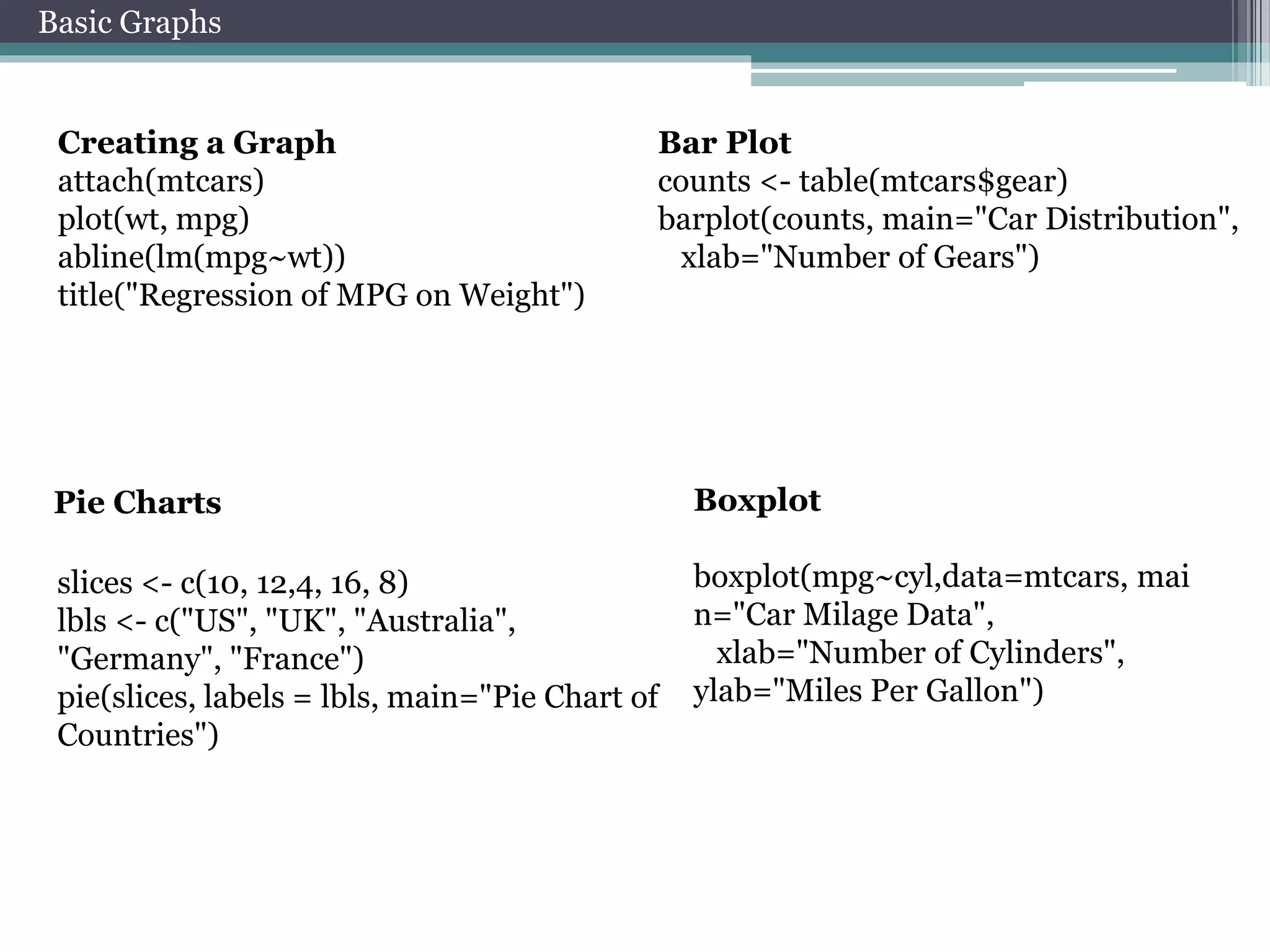
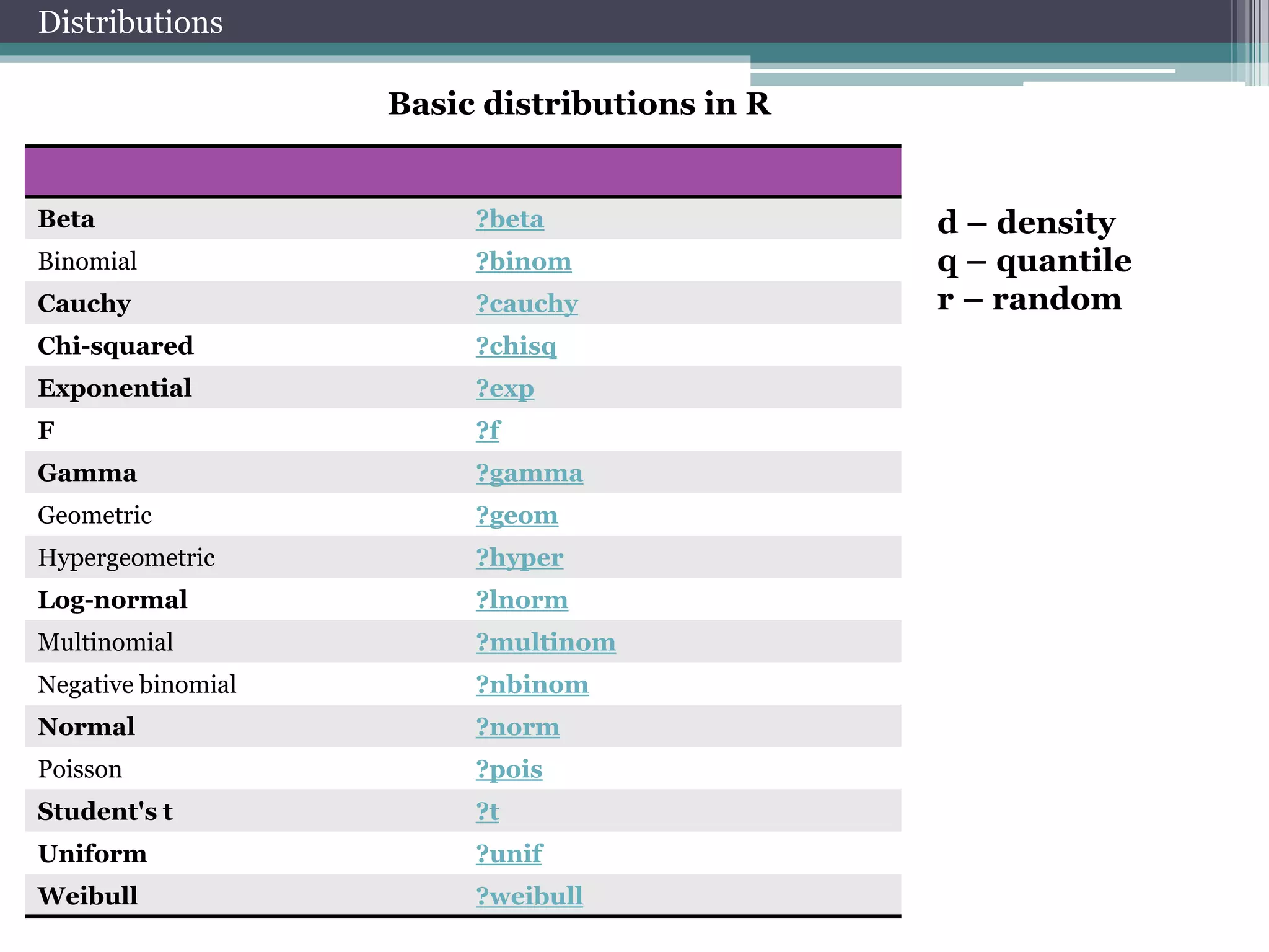
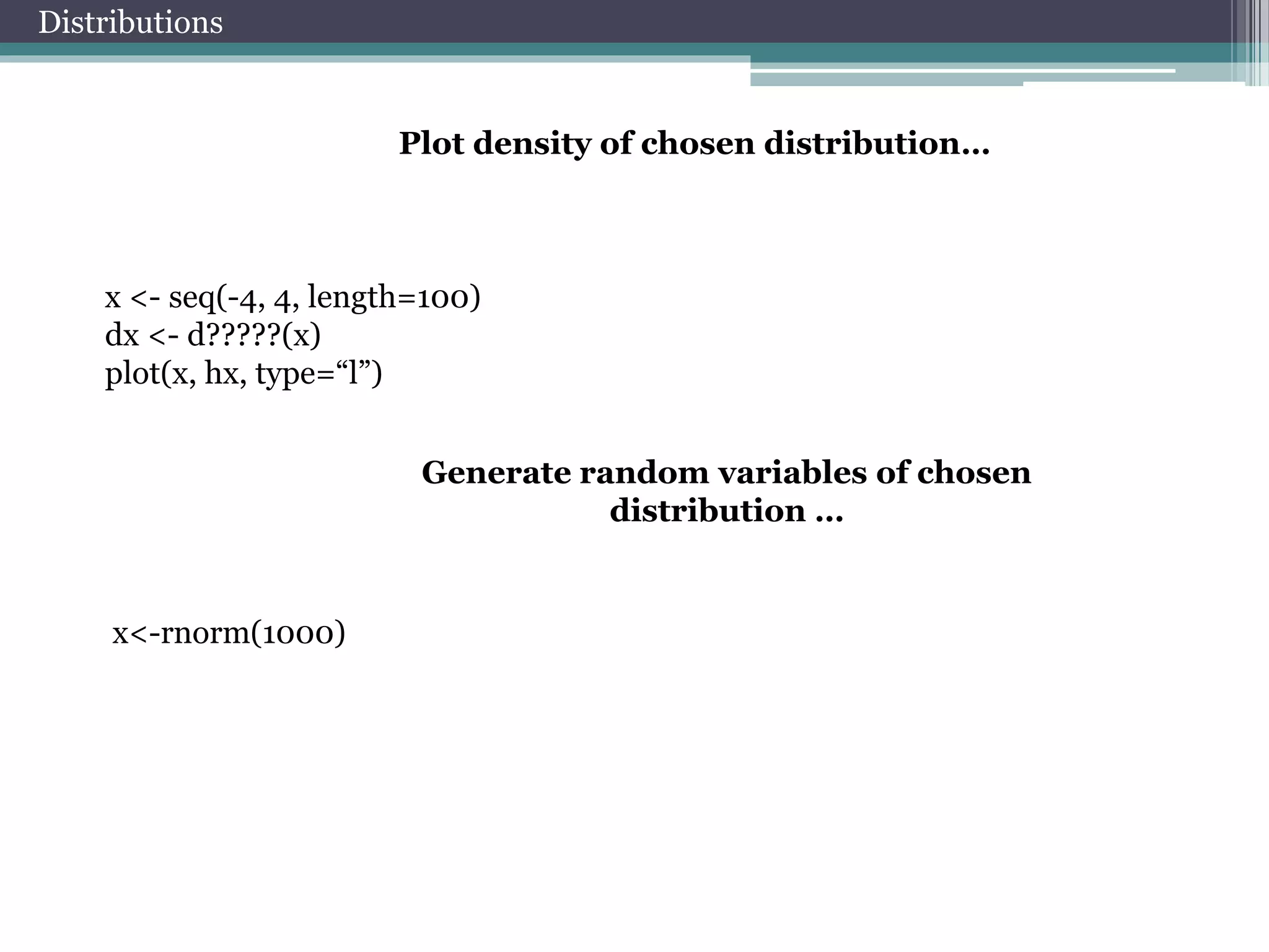
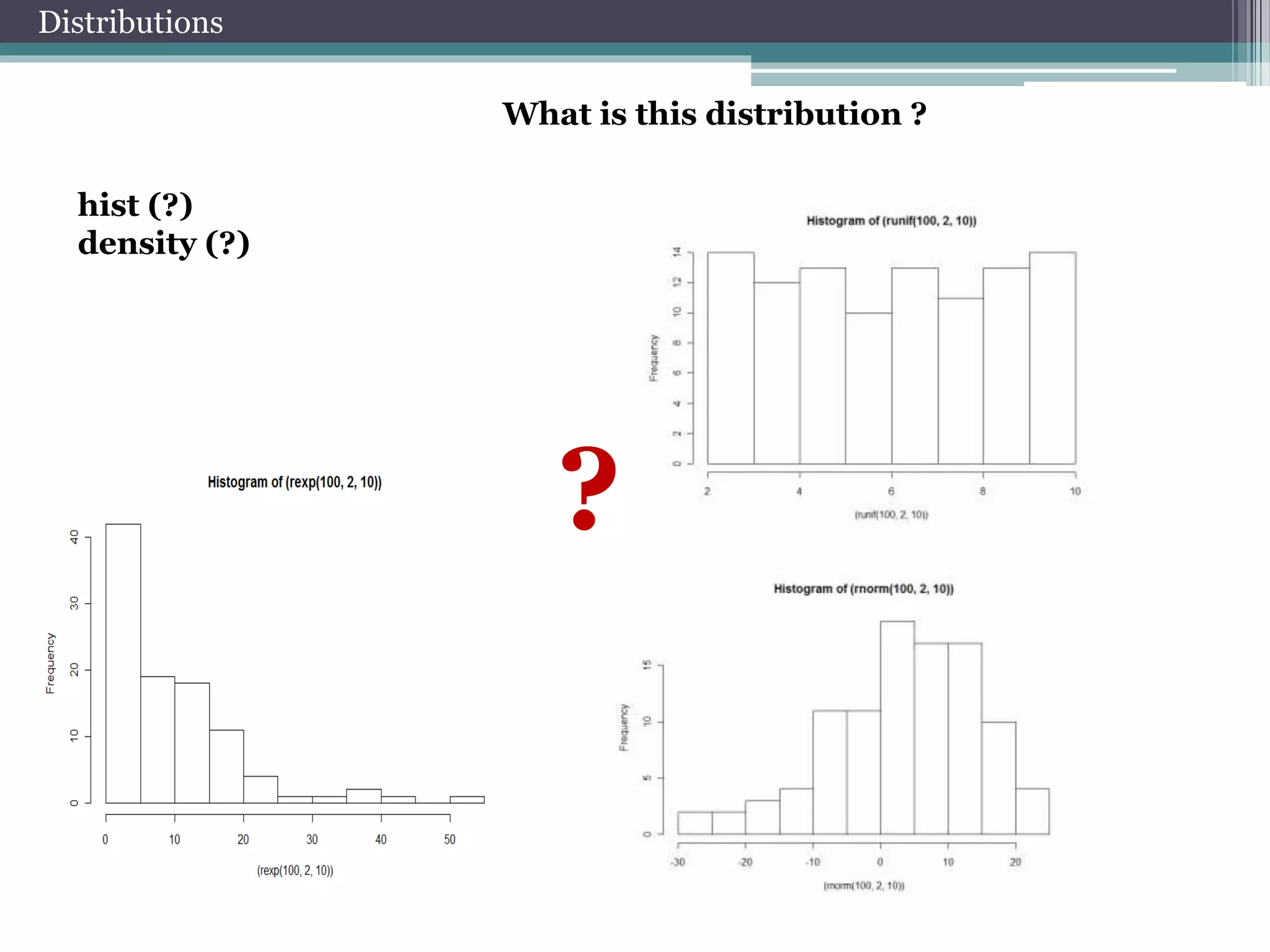
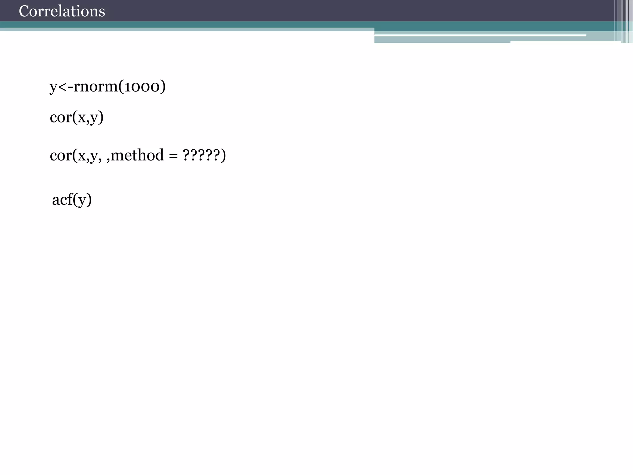
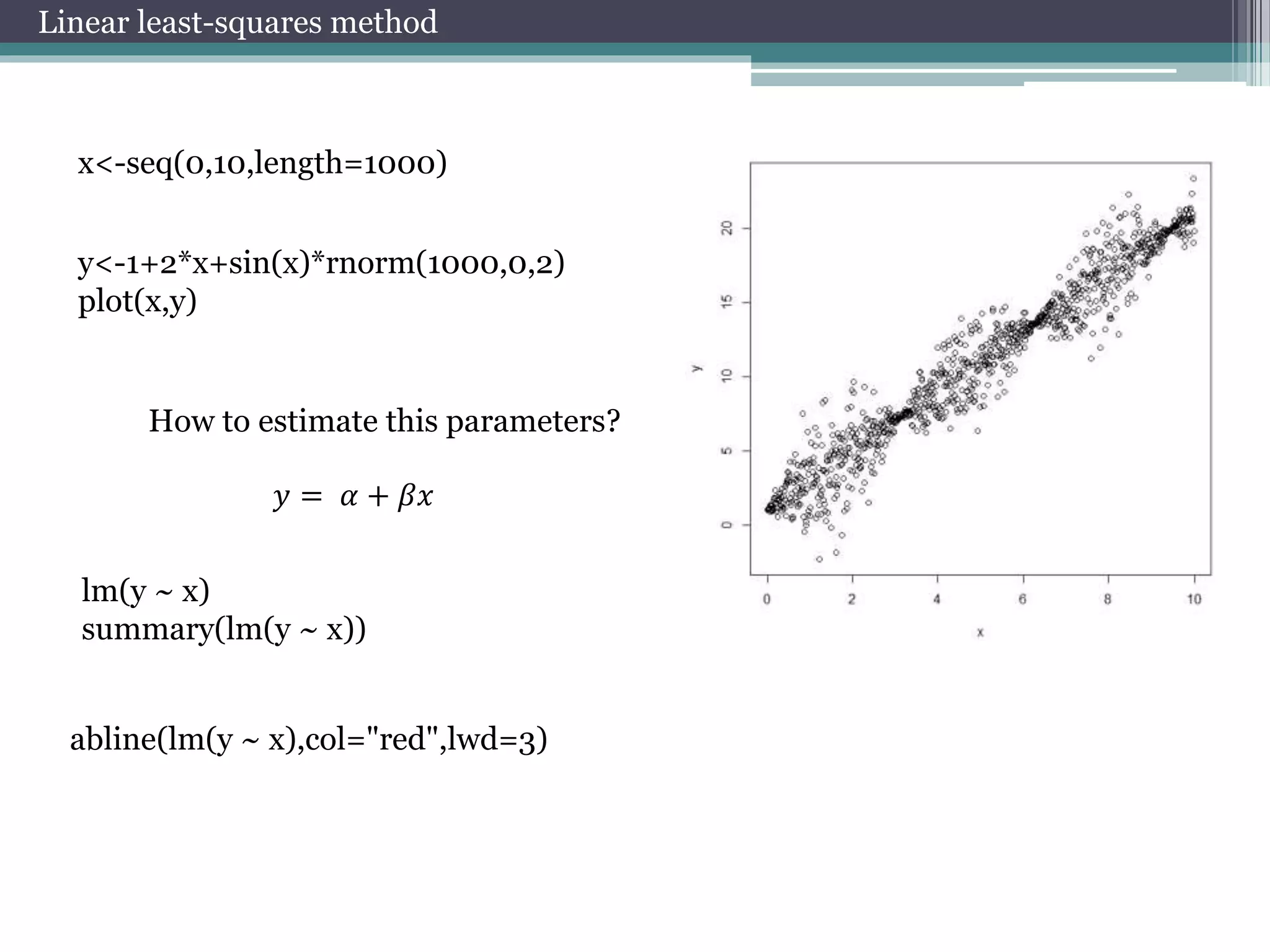
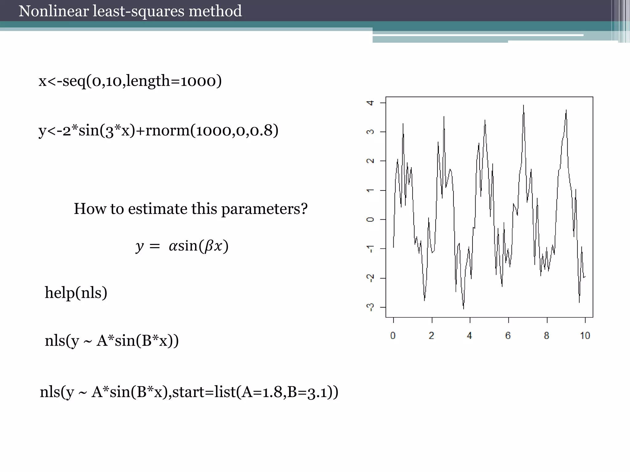
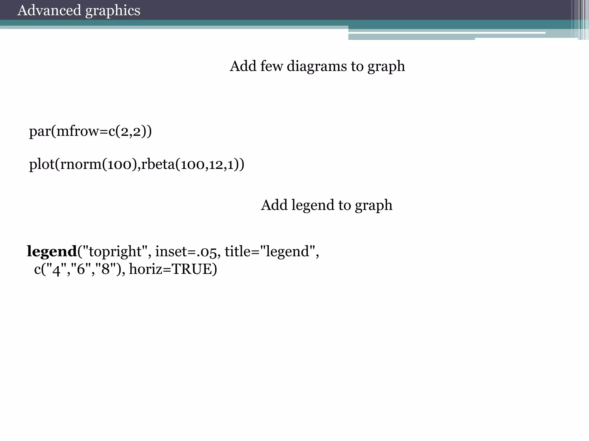
This document provides an overview of using R for financial modeling. It covers basic R commands for calculations, vectors, matrices, lists, data frames, and importing/exporting data. Graphical functions like plots, bar plots, pie charts, and boxplots are demonstrated. Advanced topics discussed include distributions, parameter estimation, correlations, linear and nonlinear regression, technical analysis packages, and practical exercises involving financial data analysis and modeling.