This document summarizes R and data mining. It introduces R language features including vectors, factors, arrays, matrices, data frames, lists, and functions. It also discusses R text mining frameworks like the 'tm' package, and preprocessing text data in R using packages like rmmseg4j, openNLP, Rstem, and Snowball. Finally, it briefly mentions high performance computing in R, network analysis in R, and statistical graphics.

1. R and Data Mining
美味书签 (AVOS China)
杨朝中

5. R and Data Mining
●
R 语言介绍
●
R 文本挖掘框架
● High Performance Computing in R
●
R 网络分析
●
统计图形

6. R and Data Mining
●
R 语言介绍
●
R 文本挖掘框架
● High Performance Computing in R
●
R 网络分析
●
统计图形

7. R 语言介绍
●
统计计算
● CRAN (Comprehensive R Archive Network)

8. R 语言介绍
●
统计计算

对象类型

统计分析模型
● CRAN (Comprehensive R Archive Network)

9. 对象类型
●
向量 (vector)
●
因子 (factor)
●
数组和矩阵 (array and matrix)
●
数据框和列表 (data.frame and list)
●
函数 (function)

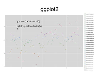
10. 向量 (vector)
> test.vector = c(1:100)
> test.vector
[1] 1 2 3 4 5 6 7 8 9 10 11 12 13 14 15 16 17 18 19 20 21 22
[23] 23 24 25 26 27 28 29 30 31 32 33 34 35 36 37 38 39 40 41 42 43 44
[45] 45 46 47 48 49 50 51 52 53 54 55 56 57 58 59 60 61 62 63 64 65 66
[67] 67 68 69 70 71 72 73 74 75 76 77 78 79 80 81 82 83 84 85 86 87 88
[89] 89 90 91 92 93 94 95 96 97 98 99 100
> test.vector[3]
[1] 3
> test.vector[1]
[1] 1
> sum(test.vector)
[1] 5050
> mean(test.vector)
[1] 50.5
> var(test.vector)
[1] 841.6667
> sd(test.vector)
[1] 29.01149

11. 因子 (factor)
> test.factor = factor(c(1,1,2,2,2,3,3,3,4,4,1,1,4,4))
> test.factor
[1] 1 1 2 2 2 3 3 3 4 4 1 1 4 4
Levels: 1 2 3 4
> levels(test.factor) = c("first","second","third","fourth")
> test.factor
[1] first first second second second third third third fourth fourth first first
[13] fourth fourth
Levels: first second third fourth
> levels(test.factor) = c("a","b","c","d")
> test.factor
[1] a a b b b c c c d d a a d d
Levels: a b c d

12. 数组 (array)
> test.array = array(rbinom(100,5,0.5),dim=c(4,5,5))
> test.array
, , 1
[,1] [,2] [,3] [,4] [,5]
[1,] 1 3 2 3 1
[2,] 4 2 2 2 2
[3,] 2 1 3 3 5
[4,] 2 2 4 2 2
> test.array[,3,]
[,1] [,2] [,3] [,4] [,5]
[1,] 2 3 4 4 2
[2,] 2 2 2 1 1
[3,] 3 2 4 3 4
[4,] 4 3 3 1 2
> test.array[3,2,]
[1] 1 2 3 1 1

13. 矩阵 (matrix)
> test.matrix = matrix(rpois(50,5),nrow=5)
> test.matrix
[,1] [,2] [,3] [,4] [,5] [,6] [,7] [,8] [,9] [,10]
[1,] 6 3 12 7 6 2 3 5 4 4
[2,] 2 5 11 3 1 4 7 2 5 5
[3,] 2 4 1 5 1 3 2 7 5 8
[4,] 4 7 5 8 4 5 3 2 6 2
[5,] 9 15 5 6 2 4 8 8 5 3
> t(test.matrix)
[,1] [,2] [,3] [,4] [,5]
[1,] 6 2 2 4 9
[2,] 3 5 4 7 15
[3,] 12 11 1 5 5
[4,] 7 3 5 8 6
[5,] 6 1 1 4 2
[6,] 2 4 3 5 4
[7,] 3 7 2 3 8
[8,] 5 2 7 2 8
[9,] 4 5 5 6 5
[10,] 4 5 8 2 3

14. 矩阵 (matix)
> test.matrix = matrix(runif(25,min=1,max=5),nrow=5)
> test.matrix
[,1] [,2] [,3] [,4] [,5]
[1,] 1.844365 2.470590 4.744482 4.693239 2.597706
[2,] 2.051089 2.954349 4.807748 3.974937 2.487159
[3,] 4.554397 2.187724 4.519553 4.916905 3.988060
[4,] 4.629351 3.770774 2.992690 4.660705 2.510643
[5,] 3.894542 3.281654 2.471337 3.484586 2.115016
> qr(test.matrix)
$qr
[,1] [,2] [,3] [,4] [,5]
[1,] -8.0591276 -6.30550129 -7.7768280 -9.2254948 -5.94547975
[2,] 0.2545051 -2.20153679 -2.8030382 -2.2409546 -0.64008014
[3,] 0.5651229 -0.83950762 -3.5747057 -2.2750825 -1.96267828
[4,] 0.5744234 -0.15061209 -0.6607485 0.7479590 0.01142934
[5,] 0.4832462 -0.07700937 -0.6148309 0.9179222 0.06790194
$rank
[1] 5
$qraux
[1] 1.22885416 1.51634534 1.43057441 1.39676050 0.06790194

15. 矩阵 (matrix)
> svd(test.matrix)
$d
[1] 17.66944239 3.22284465 1.78184517 0.61566884 0.05156261
$u
[,1] [,2] [,3] [,4] [,5]
[1,] -0.4285623 -0.55858839 0.1433838 0.6112554 0.33184518
[2,] -0.4207851 -0.46523651 0.3361892 -0.6261498 -0.31844658
[3,] -0.5179119 0.03462469 -0.8461578 -0.1172279 -0.02903471
[4,] -0.4722861 0.50932622 0.2777685 0.3687009 -0.55175807
[5,] -0.3846913 0.45926238 0.2707020 -0.2908960 0.69511911
$v
[,1] [,2] [,3] [,4] [,5]
[1,] -0.4356020 0.71976143 -0.31404796 -0.1898322 -0.39690304
[2,] -0.3666388 0.23238151 0.80369243 -0.2606880 0.31256209
[3,] -0.4958375 -0.64266729 -0.01537137 -0.4151453 -0.41053867
[4,] -0.5530530 -0.10129870 0.04863968 0.8254724 -0.01001832
[5,] -0.3522846 -0.06826158 -0.50284218 -0.2055605 0.75903264

16. 矩阵 (matrix)
> cbind(test.matrix,rep(1,times=5))
[,1] [,2] [,3] [,4] [,5] [,6]
[1,] 1.844365 2.470590 4.744482 4.693239 2.597706 1
[2,] 2.051089 2.954349 4.807748 3.974937 2.487159 1
[3,] 4.554397 2.187724 4.519553 4.916905 3.988060 1
[4,] 4.629351 3.770774 2.992690 4.660705 2.510643 1
[5,] 3.894542 3.281654 2.471337 3.484586 2.115016 1
> rbind(test.matrix, seq(1,2,length.out=5))
[,1] [,2] [,3] [,4] [,5]
[1,] 1.844365 2.470590 4.744482 4.693239 2.597706
[2,] 2.051089 2.954349 4.807748 3.974937 2.487159
[3,] 4.554397 2.187724 4.519553 4.916905 3.988060
[4,] 4.629351 3.770774 2.992690 4.660705 2.510643
[5,] 3.894542 3.281654 2.471337 3.484586 2.115016
[6,] 1.000000 1.250000 1.500000 1.750000 2.000000

17. 数据框 (data.frame)
> test.data.frame =
data.frame(id=1:10,name=letters[1:10],age=sample(c(25,23,24),size=10,replace=TRUE))
> test.data.frame
id name age
1 1 a 25
2 2 b 23
3 3 c 23
4 4 d 23
5 5 e 24
6 6 f 24
7 7 g 24
8 8 h 25
9 9 i 25
10 10 j 25
> test.data.frame$id
[1] 1 2 3 4 5 6 7 8 9 10
> test.data.frame$name
[1] a b c d e f g h i j
Levels: a b c d e f g h i j
> test.data.frame$age
[1] 25 23 23 23 24 24 24 25 25 25

18. 列表 (List)
> test.list =
list(test.vector,test.factor,test.array,test.matrix,test.data.frame)
> str(test.list)
List of 5
$ : int [1:100] 1 2 3 4 5 6 7 8 9 10 ...
$ : Factor w/ 4 levels "a","b","c","d": 1 1 2 2 2 3 3 3 4 4 ...
$ : num [1:4, 1:5, 1:5] 1 4 2 2 3 2 1 2 2 2 ...
$ : num [1:5, 1:5] 1.84 2.05 4.55 4.63 3.89 ...
$ :'data.frame': 10 obs. of 3 variables:
..$ id : int [1:10] 1 2 3 4 5 6 7 8 9 10
..$ name: Factor w/ 10 levels "a","b","c","d",..: 1 2 3 4 5 6 7 8 9 10
..$ age : num [1:10] 25 23 23 23 24 24 24 25 25 25
> test.list[4]
[[1]]
[,1] [,2] [,3] [,4] [,5]
[1,] 1.844365 2.470590 4.744482 4.693239 2.597706
[2,] 2.051089 2.954349 4.807748 3.974937 2.487159
[3,] 4.554397 2.187724 4.519553 4.916905 3.988060
[4,] 4.629351 3.770774 2.992690 4.660705 2.510643
[5,] 3.894542 3.281654 2.471337 3.484586 2.115016

19. 函数 (function)
> test.function = function(x) factorial(x)
> test.function(3)
[1] 6
>lapply(test.vector[31:35],test.function)
[[1]]
[1] 8.222839e+33
[[2]]
[1] 2.631308e+35
[[3]]
[1] 8.683318e+36
[[4]]
[1] 2.952328e+38
[[5]]
[1] 1.033315e+40

20. 统计分析模型
●
回归分析
●
方差分析
●
判别分析
●
聚类分析
●
主成分分析
●
因子分析
●
连续系统模拟、离散系统模拟

21. R 语言介绍
●
统计计算
● CRAN (Comprehensive R Archive Network)

22. CRAN
● CRAN Task Views
● Natural Language Processing
● Machine Learning & Statistical Learning
● High-Performance and Parallel Computing with R
● gRaphical Models in R
● Graphic displays

23. R and Data Mining
●
R 语言介绍
●
R 文本挖掘框架
● High Performance Computing in R
●
R 网络分析
●
统计图形

24. R 文本挖掘框架

25. ‘tm’ package UML 类图

26. Text Preprocessing in R
●
数据导入： Corpus 、 PlainTextDocument 、 tm_map
●
中文分词： rmmseg4j
●
英文词干提取： Rstem 、 Snowball 、 RWeka
●
英文句子识别： openNLP
●
英文同义词： wordnet
●
构造基于 tf-idf 的文档单词矩阵：
DocumentTermMatrix 、 weightTfIdf

27. Preprocessing
library(tm)
library(rmmseg4j)
library(openNLP)
library(Rstem)
library(Snowball)
cor = Corpus(DirSource("~/work/text-mining/20news-bydate-test/1000/"),
readerControl=list(reader=readPlain))
cwsed = tm_map(cor, function(x){
PlainTextDocument(mmseg4j(as.character(x), method="maxword"),
id=ID(x))
})
dtm = DocumentTermMatrix(cwsed, control=list(weighting = function(x){
weightTfIdf(x)
},wordLengths=c(1,Inf)))

28. 文本聚类
降维处理
++++++++++++++++++++++++++++++++++++++++++
> nTerms(dtm)
[1] 103757
> dtm2 = removeSparseTerms(dtm, 0.9)
> nTerms(dtm2)
[1] 709
++++++++++++++++++++++++++++++++++++++++++
聚类
++++++++++++++++++++++++++++++++++++++++++
km = kmeans(as.matrix(dtm2), centers=5, iter.max=10)
dbscan?
spectral clustering?

29. Cluster validation
● Internal measures
● Stability measures
● Biological

30. Internal measures
● Connectivity
● Silhouette Width
● Dunn Index

31. Stability measures
● Average Proportion of Non-overlap(APN)
● Average Distance (AD)

32. Stability measures
● Average Distance between Means (ADM)
● Figure of Merit (FOM)

33. Biological
● Biological Homogeneity Index (BHI)
● Biological Stability Index (BSI)

34. Cluster validation
library(tm)
library(kernlab)
library(clValid)
intern=clValid(as.matrix(dtm2),2:10,clMethods=c("hierarchical","kmeans","pa
m"),validation="internal",maxitems=3000)
summary(intern)
op <- par(no.readonly=TRUE)
par(mfrow=c(2,2),mar=c(4,4,3,1))
plot(intern, legend=FALSE)
legend("right", clusterMethods(intern), col=1:9, lty=1:9, pch=paste(1:9))
par(op)

36. 文本分类
●
朴素贝叶斯
●
支持向量机 (Support Vector Machine)
台湾大学 林智仁
Libsvm(e1071)
Liblinear(LiblinearR)

37. Evaluation and Acurracy
improvement
● Cross validation
● Bootstrap
● Ensemble Method

38. R and Data Mining
●
R 语言介绍
●
R 文本挖掘框架
● High Performance Computing in R
●
R 网络分析
●
统计图形

39. High Performance Computing in R
● Parallel Computing
Rmpi 、 snowfall 、 snowFT 、
parallel(>=R 2.14) 、 Rhadoop
● Large memory and out-of-memory data
ff 、 HadoopStreaming
● Easier interfaces for Compiled code
Rcpp 、 Rjava 、 inline
● Profiling tools
profr 、 proftools

40. Rhadoop
http://www.revolutionanalytics.com/

41. Rhadoop
● Rmr2
mapreduce 、 from.dfs 、 to.dfs 、 keyval
● Rhdfs
hdfs.file 、 hdfs.close 、 hdfs.exists 、 hdfs.cp
hdfs.read
● Rhbase
hb.new.table 、 hb.delete.table 、 hb.insert 、
hb.get

42. k-medios.iter =
function(points, distfun,ncenters,centers = NULL) {
from.dfs(mapreduce(input = points,
map =
if (is.null(centers)) {
function(k,v) keyval(sample(1:ncenters,1),v)
}
else {
function(k,v) {
distances = apply(centers, 1, function(c) distfun(c,v))
keyval(centers[which.min(distances),], v)
}
},
reduce = function(k,vv) keyval(NULL, iter.center(vv)),
structured = T))
}

43. Parallel computing
library(snowfall)
library(tm)
library(kernlab)
svm_parallel =
function(dtm){
sfInit(parallel=TRUE, cpus=4, type="MPI")
data = as.data.frame(inspect(dtm))
data$type = factor(rep(1:5, times=c(500,500,500,500,564)))
levels(data$type) = c('sports','tech','news','education','learning')
sub = sample(c(0,1,2,3,4), size=2564, replace=T)
wrapper = function(x){
if(require(kernlab)){
ksvm(type ~., data=x)
}
}
ksvm.models =
sfLapplyLB(c(data[sub==0,],data[sub==1,],data[sub==2,],data[sub==3,],data[sub==4,]),
wrapper)
sfStop()
ksvm.models
}

44. Parallel computing
> library(parallel)
> cl =
makeCluster(detectCores(logical=FALSE))
> parLapplyLB(cl, 46:50, test.function)
[[1]]
[1] 5.502622e+57
[[2]]
[1] 2.586232e+59
[[3]]
[1] 1.241392e+61
[[4]]
[1] 6.082819e+62
[[5]]
[1] 3.041409e+64

45. R and Data Mining
●
R 语言介绍
●
R 文本挖掘框架
● High Performance Computing in R
●
R 网络分析
●
统计图形

46. library(igraph)
g <- graph.full(6,
directed=FALSE)
plot(g)

47. library(igraph)
g <- graph.ring(10,
directed=FALSE)
plot(g)

48. library(igraph)
g <- graph.star(16, mode = c("undirected"), center = 1)
plot(g)

49. library(igraph)
g <-
graph(c(1,2,4,5,3,4,5,6),directed=FALSE)
plot(g)

50. library(igraph)
M <- matrix(runif(100),nrow=10)
g <- graph.adjacency(M>0.9)
plot(g)

51. > M[,1:5]
[,1] [,2] [,3] [,4] [,5] [,6] [,7] [,8]
[1,] 0.44746867 0.9753915 0.6890068 0.8500356 0.5812459
[2,] 0.10004725 0.9870645 0.9322102 0.6834764 0.8518852
[3,] 0.04882503 0.1599767 0.5268769 0.7756217 0.5713700
[4,] 0.91988082 0.4018993 0.3562261 0.7624379 0.1849250
[5,] 0.43281897 0.6032613 0.8240209 0.3340224 0.7189334
[6,] 0.87971431 0.9331585 0.4483813 0.4743045 0.5121772
[7,] 0.04519996 0.1875099 0.5615725 0.5913464 0.9487314
[8,] 0.78936780 0.6904077 0.6834867 0.2760950 0.1559759
[9,] 0.13621689 0.5607899 0.2745078 0.7246721 0.1932709
[10,] 0.54878255 0.4730136 0.7992216 0.4186087 0.2547914
> M[,1:5] > 0.9
[,1] [,2] [,3] [,4] [,5] [,6] [,7] [,8]
[1,] FALSE TRUE FALSE FALSE FALSE
[2,] FALSE TRUE TRUE FALSE FALSE
[3,] FALSE FALSE FALSE FALSE FALSE
[4,] TRUE FALSE FALSE FALSE FALSE
[5,] FALSE FALSE FALSE FALSE FALSE
[6,] FALSE TRUE FALSE FALSE FALSE
[7,] FALSE FALSE FALSE FALSE TRUE
[8,] FALSE FALSE FALSE FALSE FALSE
[9,] FALSE FALSE FALSE FALSE FALSE
[10,] FALSE FALSE FALSE FALSE FALSE

52. library(igraph)
g1 <- graph.full(6, directed=FALSE)
g2 <- graph(c(6,7,7,8,8,9,9,10,9,7,11,12,12,8),
directed=FALSE)
g <- graph.union(g1, g2)
plot(g)

53. > V(g)
Vertex sequence:
[1] 1 2 3 4 5 6 7 8 9 10 11 12
> degree(g)
[1] 5 5 5 5 5 6 3 3 3 1 1 2
> V(g)[degree(g)>1]
Vertex sequence:
[1] 1 2 3 4 5 6 7 8 9 12
> graph.dfs(g, 9)
$order
[1] 9 7 6 1 2 3 4 5 8 12 11 10
> graph.bfs(g, 9)
$order
[1] 9 7 8 10 6 12 1 2 3 4 5 11

54. 网络分析
● igraph
● graph
● network
● sna

55. R and Data Mining
●
R 语言介绍
●
R 文本挖掘框架
● High Performance Computing in R
●
R 网络分析基本
●
统计图形

56. 统计图形
Statistical graphics is, or should be, an
transdisciplinary field informed by scientific,
statistical,computing, aesthetic, psychological
and sociological considerations.[Leland
Wilkinson, The Grammar of Graphics]

57. The grammar of Graphics
In brief, the grammar tells us that the statistical
graphic is a mapping from data to aesthetic
attributes(color, shape,size) of geometric
objects(points, lines, bars).

58. 直方图 (hist)

59. 条形图 (barplot)

60. 散点图 (plot)
> x=seq(from=-pi,to=pi,length.out=100)
> y=sin(x)
> plot(x, y, col="blue")

61. 概率密度曲线
> x=seq(from=-pi,to=pi,length.out=100)
> y = dnorm(x)
> plot(x, y, col="blue")

62. 颜色等高图

63. 散点图矩阵

64. 矩阵图 (matplot)
matplot(test.matrix,type="b")

65. 高级绘图程序
● lattice
● ggplot2
An implementation of the grammar of graphics
in R

66. ggplot2
●
Data( 数据 ) 和 Mapping( 映射 )
●
Geom( 几何对象 )
●
Stat( 统计变换 )
●
Scale( 标度 )
●
Coord( 坐标系统 )
●
Facet( 分面 )
●
Layer( 图层 )

67. ggplot2
●
测试数据
> str(mpg)
'data.frame': 234 obs. of 11 variables:
$ manufacturer: Factor w/ 15 levels "audi","chevrolet",..: 1 1 1 1 1 1 1 1 1 1 ...
$ model : Factor w/ 38 levels "4runner 4wd",..: 2 2 2 2 2 2 2 3 3 3 ...
$ displ : num 1.8 1.8 2 2 2.8 2.8 3.1 1.8 1.8 2 ...
$ year : int 1999 1999 2008 2008 1999 1999 2008 1999 1999 2008 ...
$ cyl : int 4 4 4 4 6 6 6 4 4 4 ...
$ trans : Factor w/ 10 levels "auto(av)","auto(l3)",..: 4 9 10 1 4 9 1 9 4 10 ...
$ drv : Factor w/ 3 levels "4","f","r": 2 2 2 2 2 2 2 1 1 1 ...
$ cty : int 18 21 20 21 16 18 18 18 16 20 ...
$ hwy : int 29 29 31 30 26 26 27 26 25 28 ...
$ fl : Factor w/ 5 levels "c","d","e","p",..: 4 4 4 4 4 4 4 4 4 4 ...
$ class : Factor w/ 7 levels "2seater","compact",..: 2 2 2 2 2 2 2 2 2 2 ...

68. ggplot2
> library(ggplot2)
> p <- ggplot(data=mpg,
mapping=aes(x=cty,y=hwy))
> p + geom_point()

69. ggplot2
> p <- ggplot(data=mpg,
mapping=aes(x=cty,y=hwy,colour=factor(year)))
> p + geom_point()

70. ggplot2
> p + geom_point() + stat_smooth()

71. ggplot2
> p + geom_point(mapping=aes(size=displ)) +
stat_smooth()

72. ggplot2
> p + geom_point(mapping=aes(size=displ)) + stat_smooth() +
coord_cartesian(xlim=c(20,30),ylim=c(0,40))

73. ggplot2
> p + geom_point(mapping=aes(size=displ)) + stat_smooth() +
facet_wrap(~year,ncol=2)

74. ggplot2
qplot(x,y,colour=factor(y)
)

75. ggplot2
y = sin(x) + rnorm(100)
qplot(x,y,colour=factor(y)
)

76. ggplot2
plotmatrix(data,mapping=aes(),colour="blue")

77. R 中文博客
●
肖凯
http://xccds1977.blogspot.jp
●
刘思喆
统计之都 R 语言版版主
http://cos.name/cn/
●
谢益辉
http://yihui.name/

78. 国外网站
●
数据科学家 twitter
Big Data: Experts to Follow on Twitter
●
R 语言相关论文或书籍
Journal of Statistical Software
● R and Data Mining
http://www.rdatamining.com/
● R-project search
http://www.rseek.org/