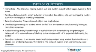
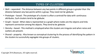
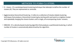
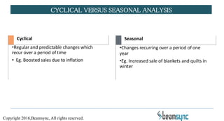
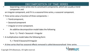
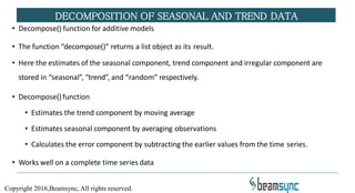
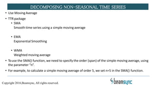
The document discusses various clustering techniques such as hierarchical, partitioned, exclusive, overlapping, fuzzy, and complete clustering. It also provides insights into time series analysis, including its components (trend, seasonal, cyclical, and irregular variations) and methods for predicting future values. Additionally, the document highlights techniques for decomposing time series data to analyze its constituent components effectively.

1. BUSINESS ANALYTICS FOUNDATION WITH R
TOOLS
Lesson 4 - Predictive Modeling Techniques
Copyright 2016,Beamsync, All rights reserved.

2. • Hierarchical : Also known as nesting clusters as it also clusters to exist within bigger clusters to form
a tree.
• Partitioned clustering : Its simply a division of the set of data objects into non-overlapping clusters
such that each object is in exactly one subset.
• Exclusive clustering: They assign each object to a single cluster.
• Overlapping clustering : Its used to reflect the fact that an object can simultaneously belong to
more than one group.
• Fuzzy clustering : Every object belongs to every cluster with a membership weight that goes
between 0 – if it absolutely doesn’t belong to that cluster and 1 – if it absolutely belongs to the
cluster.
• Complete clustering : It performs a hierarchical cluster analysis using a set of dissimilarities on n
objects that are being clustered. They tend to find compact clusters of an approximately equal
diameters.
TYPES OF CLUSTERING
Copyright 2016,Beamsync, All rights reserved.

3. • Well – separated : The distance between any two points in different groups is greater than the
distance between any two points within a group. They need not be globular.
• Prototype – based : The prototype of a cluster is often a centroid for data with continuous
attributes. Such clusters tend to be globular.
• Graph – based : When data is represented as a graph where nodes are the objects and links
represent connection among the objects. They tend to be globular.
• Density – based : This method is employed when the clusters are irregular and when noise and
outliers are present.
• Shared – property : Also known as conceptual clustering its the process of identifying the pattern in
the clusters to successfully segregate into groups of clusters.
TYPES OF CLUSTERS
Copyright 2016,Beamsync, All rights reserved.

4. • K – means : It’s a prototype based clustering technique that attempts to define the number of
clusters (K). They are represented as centroids.
• Agglomerative Hierarchical Clustering : It refers to a collection of closely related clustering
techniques that produce a hierarchical clustering by starting with each point as singleton cluster
and repeatedly merging the closest clusters until a single, all encompassing cluster remains.
• DBSCAN : It’s a density based clustering algorithm that produces a partitioned clustering, in which
number of clusters is automatically determined by the algorithm.
METHODS TO FORM CLUSTERS.
Copyright 2016,Beamsync, All rights reserved.

5. • Time series data is an ordered sequence of observations on a quantitative variable measured over
an equally spaced time interval.
• Time series are used in statistics, signal processing, pattern recognition, econometrics, mathematic
finance, weather forecasting, earthquake prediction electroencephalography, control engineering,
astronomy , communications engineering and other places.
• The ultimate objective of time series is –we want to predict the future value of variable under
consideration.
• Time series analysis is
• a set of methods used for analyzing time series data
• and forecasting the future value of the variable under consideration.
• In time series analysis it is assumed that the data consist of set of identifiable components and
random errors which usually makes the pattern difficult to identify.
• E.g. Consider a store that sells blankets and quilts. Then the store will observe sale of the quilts to
be maximum during the winter season. This case comes under seasonal variation.
TIME SERIES
Copyright 2016,Beamsync, All rights reserved.

6. • Long term trend – The smooth long term direction of time series where the data can increase or
decrease in some pattern.
• Seasonal variation – Patterns of change in a time series within a year which tends to repeat every
year.
• Cyclical variation – Its much alike seasonal variation but the rise and fall of time series over periods
are longer than one year.
• Irregular variation – Any variation that is not explainable by any of the three above mentioned
components. But that doesn’t explain the variations to be random. They can be classified into –
stationary and non – stationary variation.
• When the data neither increases nor decreases, i.e. its completely random its called stationary
variation.
• When the data has some explainable portion remaining and can be analyzed further then such
case is called non – stationary variation.
COMPONENTS OF TIME SERIES ANALYSIS
Copyright 2016,Beamsync, All rights reserved.

7. CYCLICAL VERSUS SEASONAL ANALYSIS
Cyclical
•Regular and predictable changes which
recur over a period of time
• Eg. Boosted sales due to inflation
Seasonal
•Changes recurring over a period of one
year
•Eg. Increased sale of blankets and quilts in
winter
Copyright 2016,Beamsync, All rights reserved.

8. • Separating a time series into its constituent components, which are usually a trend
component and
an irregular component, and if it is a seasonal time series, a seasonal component.
• Time series value a function of three components –
• Trendcomponent,
• Seasonal component
• irregular or error component.
• An additive decomposition model takes the following
form: Yt = Trend + Seasonal + Irregular
• A multiplicative model takes the following form:
Yt = Trend X Seasonal XIrregular
• A time series that has seasonal effects removed is called deseasonalised time series.
DECOMPOSITION OF TIME SERIES
Copyright 2016,Beamsync, All rights reserved.

9. • Decompose() function for additive models
• The function “decompose()” returns a list object as its result.
• Here the estimates of the seasonal component, trend component and irregular component are
stored in “seasonal”, “trend”, and “random” respectively.
• Decompose()function
• Estimates the trend component by moving average
• Estimates seasonal component by averaging observations
• Calculates the error component by subtracting the earlier values from the time series.
• Works well on a complete time series data
DECOMPOSITION OF SEASONAL AND TREND DATA
Copyright 2016,Beamsync, All rights reserved.

10. • Use MovingAverage
• TTR package
• SMA
Smooth time series using a simple moving average
• EMA
Exponential Smoothing
• WMA
Weighted moving average
• Touse the SMA() function, we need to specify the order (span) of the simple moving average, using
the parameter “n”.
• For example, to calculate a simple moving average of order 5, we set n=5 in the SMA() function.
DECOMPOSING NON-SEASONAL TIME SERIES
Copyright 2016,Beamsync, All rights reserved.

11. Thank You
Beamsync is top training institute for business analytics course in Bangalore.
Beamsync is also providing certification along with training course. For more
details click here: http://beamsync.com/business-analytics-training-bangalore/
Copyright 2016,Beamsync, All rights reserved.