Downloaded 15 times


![> class(model1)
[1] "lm"
the output from the lm function is an object of class
lm. An object of class "lm" is a list containing at least
the following components:](https://image.slidesharecdn.com/day5-1-linear-models-170531132054/75/11-Linear-Models-15-2048.jpg)
![> class(model1)
[1] "lm"
the output from the lm function is an object of class
lm. An object of class "lm" is a list containing at least
the following components:
coefficients - a named vector of coefficients
residuals - the residuals, that is response minus fitted values.
fitted.values - the fitted mean values.
rank - the numeric rank of the fitted linear model.
weights - (only for weighted fits) the specified weights.
df.residual -the residual degrees of freedom.
call - the matched call.
terms - the terms object used.
contrasts - (only where relevant) the contrasts used.
xlevels -(only where relevant) a record of the levels of the factors
used in fitting.
offset- the offset used (missing if none were used).
y - if requested, the response used.
x- if requested, the model matrix used.
model - if requested (the default), the model frame used.
na.action - (where relevant) information returned by model.frame on
the special handling of NAs.](https://image.slidesharecdn.com/day5-1-linear-models-170531132054/75/11-Linear-Models-16-2048.jpg)
![class(model1)
[1] "lm"
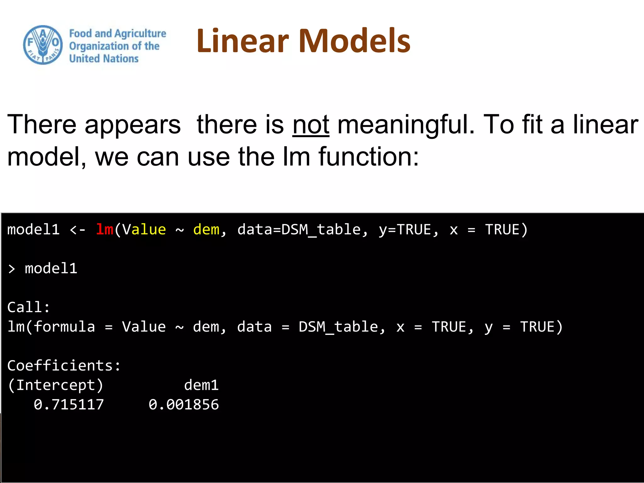
model1$coefficients
(Intercept) dem1
0.715116901 0.001856089
> formula(model1)
Value ~ dem1
the output from the lm function is an object of class
lm. An object of class "lm" is a list containing at least
the following components:](https://image.slidesharecdn.com/day5-1-linear-models-170531132054/75/11-Linear-Models-17-2048.jpg)
![head(residuals(model1))
1 2 3 4 5 6
6.8445691 -1.2674728 -0.7045624 -0.5960802 -1.1628119 -1.1990168
names(summary(model1))
[1] "call" "terms" "residuals" "coefficients"
[5] "aliased" "sigma" "df" "r.squared"
[9] "adj.r.squared" "fstatistic" "cov.unscaled"
Here is a list of what is available from the summary
function for this model:](https://image.slidesharecdn.com/day5-1-linear-models-170531132054/75/11-Linear-Models-18-2048.jpg)
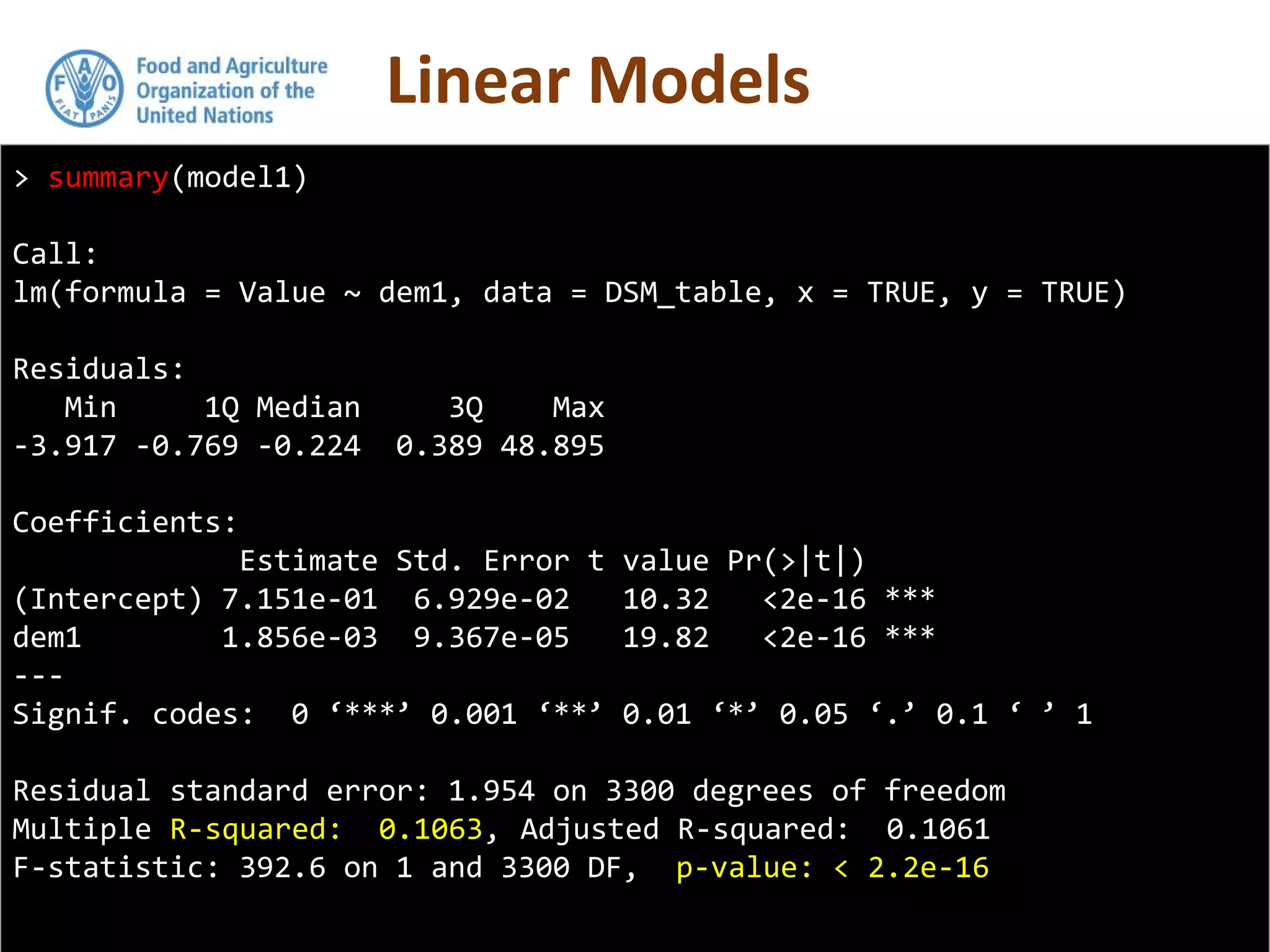
![summary(model1)[[4]]
Estimate Std. Error t value Pr(>|t|)
(Intercept) 0.715116901 6.928677e-02 10.32112 1.333183e-24
dem1 0.001856089 9.367314e-05 19.81452 1.188533e-82
summary(model1)[[7]]
[1] 2 3300 2
To extract some of the information from the
summary which is of a list structure, we can use:](https://image.slidesharecdn.com/day5-1-linear-models-170531132054/75/11-Linear-Models-19-2048.jpg)
![> summary(model1)[["r.squared"]]
[1] 0.1063245
> summary(model1)[[8]]
[1] 0.1063245
What is the RSquared of model1?](https://image.slidesharecdn.com/day5-1-linear-models-170531132054/75/11-Linear-Models-20-2048.jpg)
![> summary(model1)[["r.squared"]]
[1] 0.1063245
> summary(model1)[[8]]
[1] 0.1063245
What is the RSquared of model1?](https://image.slidesharecdn.com/day5-1-linear-models-170531132054/75/11-Linear-Models-21-2048.jpg)
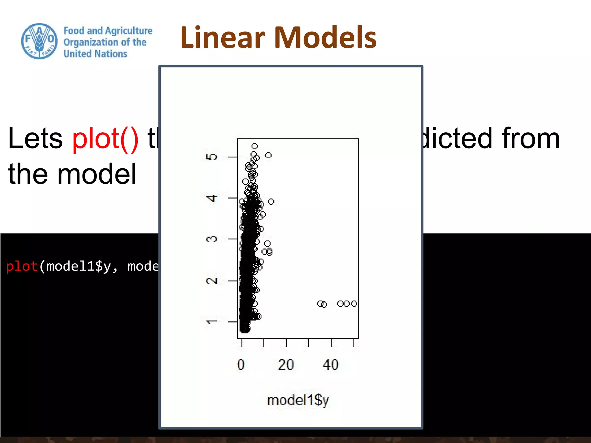
![head(predict(model1))
1 2 3 4 5 6
5.034235 4.757678 3.022235 2.532228 2.502530 3.484401
head(DSM_table$Value)
[1] 11.878804 3.490205 2.317673 1.936148 1.339719 2.285384
head(residuals(model1))
1 2 3 4 5 6
6.8445691 -1.2674728 -0.7045624 -0.5960802 -1.1628119 -1.1990168
head(model2$residuals)
1 2 3 4 5 6
7.3395541 -1.1690560 -0.5363049 -1.2854938 -1.9692882 -1.5173124
> head(model2$fitted.values)
1 2 3 4 5 6
4.539250 4.659261 2.853978 3.221641 3.309007 3.802697](https://image.slidesharecdn.com/day5-1-linear-models-170531132054/75/11-Linear-Models-22-2048.jpg)
![model2subset <-DSM_table2[, c("Value", "slp", "prec", "dem")]
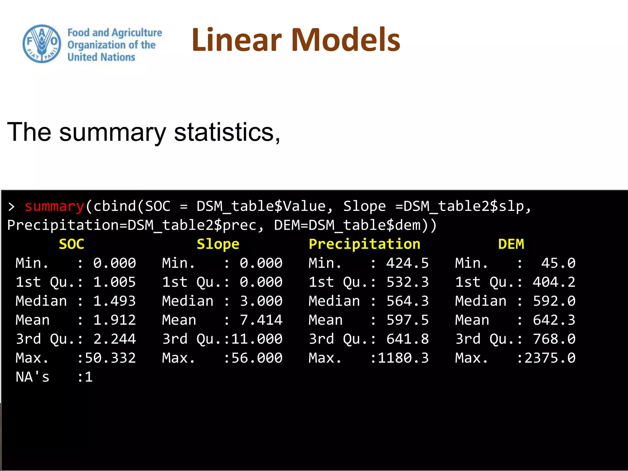
summary(model2subset)
Value slp prec dem
Min. : 0.000 Min. : 0.000 Min. : 424.5 Min. : 45.0
1st Qu.: 1.005 1st Qu.: 0.000 1st Qu.: 532.3 1st Qu.: 404.2
Median : 1.493 Median : 3.000 Median : 564.3 Median : 592.0
Mean : 1.912 Mean : 7.414 Mean : 597.5 Mean : 642.3
3rd Qu.: 2.244 3rd Qu.:11.000 3rd Qu.: 641.8 3rd Qu.: 768.0
Max. :50.332 Max. :56.000 Max. :1180.3 Max. :2375.0
NA's :1
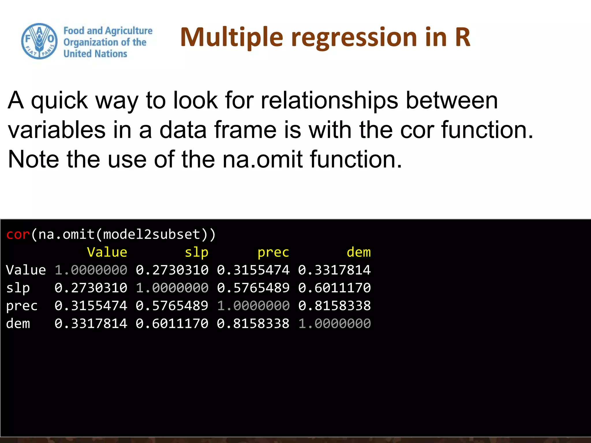
We will regress SOC on Precipitation,
Slope and Elevation. First lets subset these
data out, then get their summary statistics](https://image.slidesharecdn.com/day5-1-linear-models-170531132054/75/11-Linear-Models-24-2048.jpg)
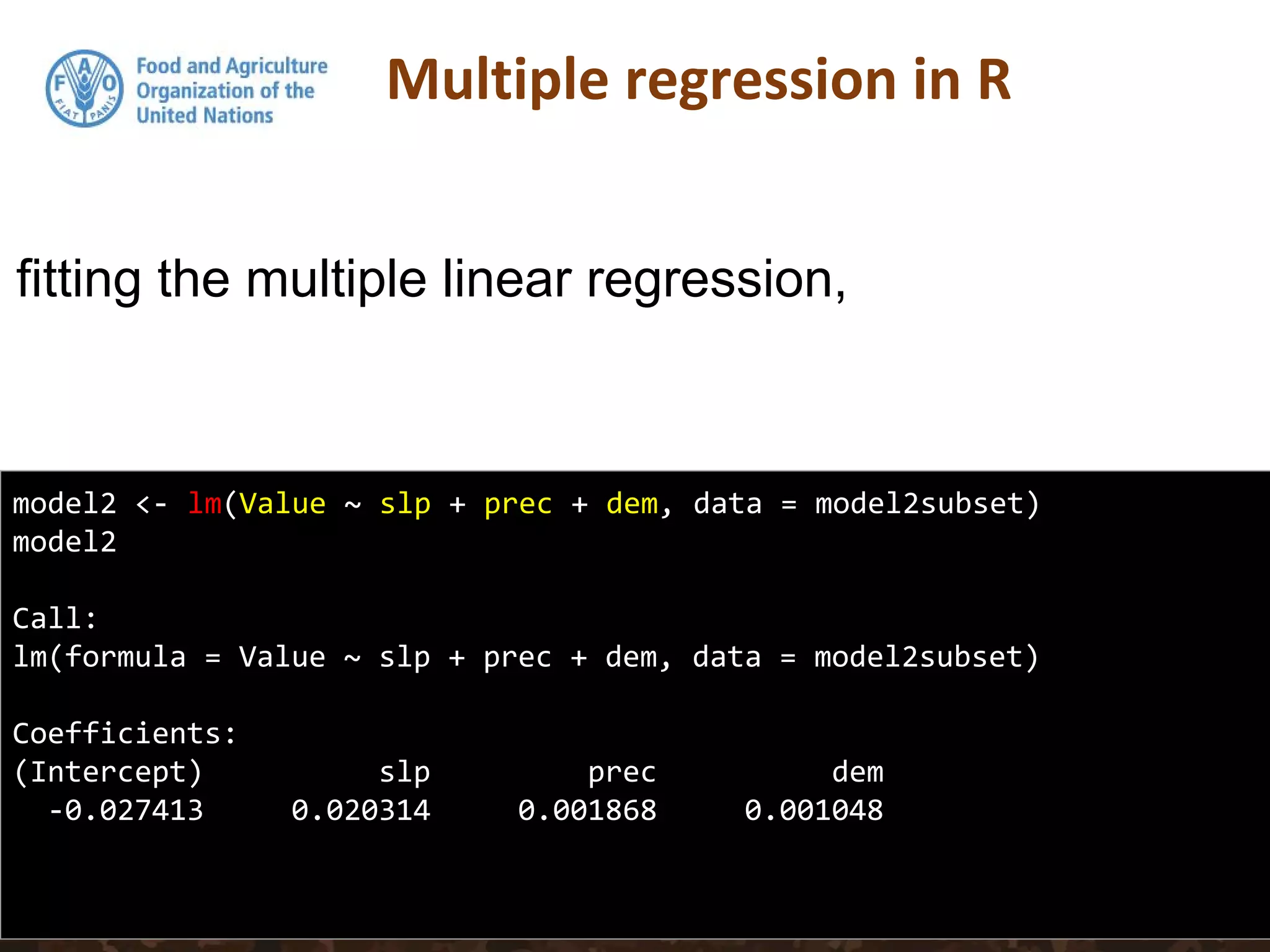
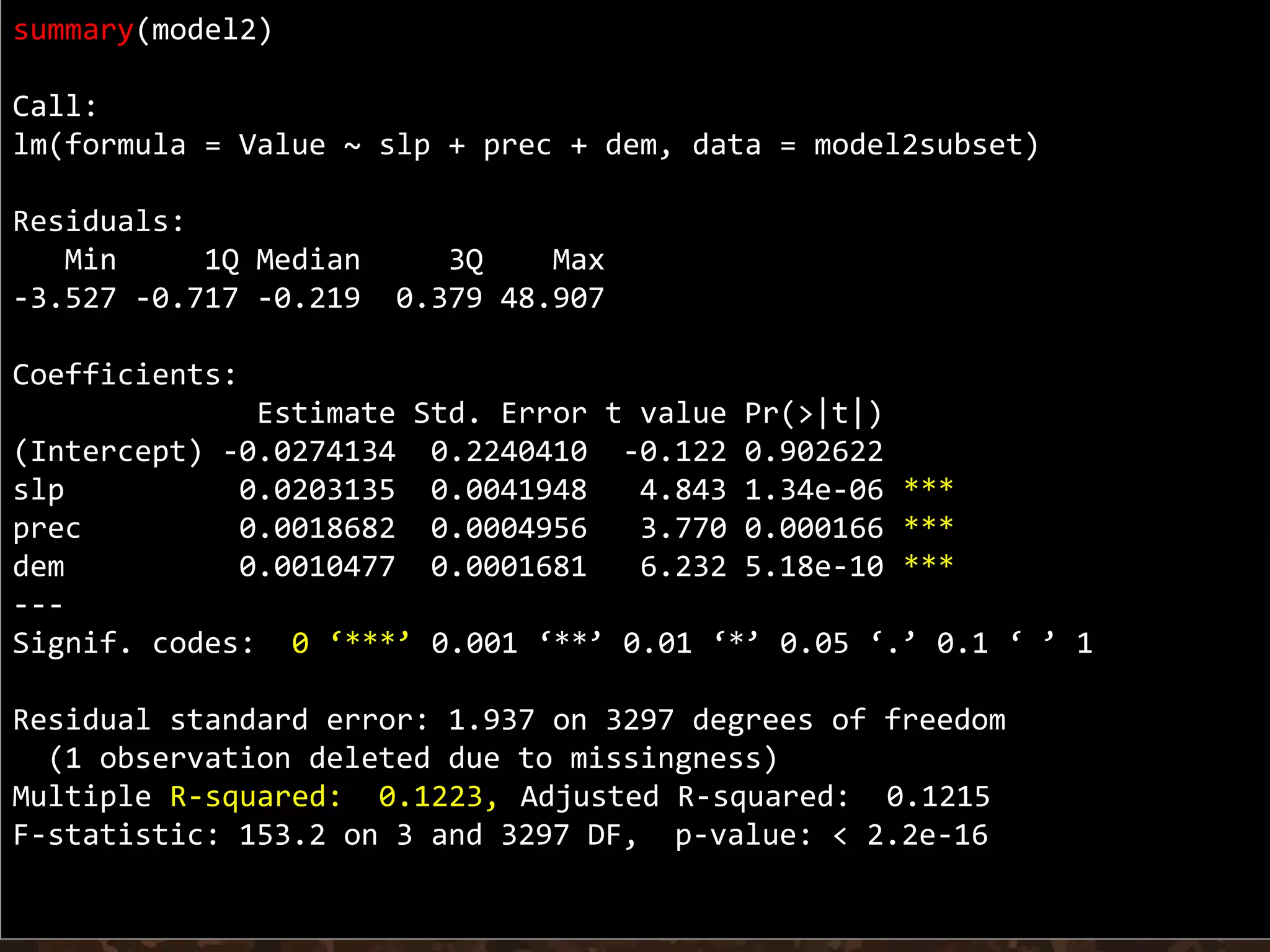

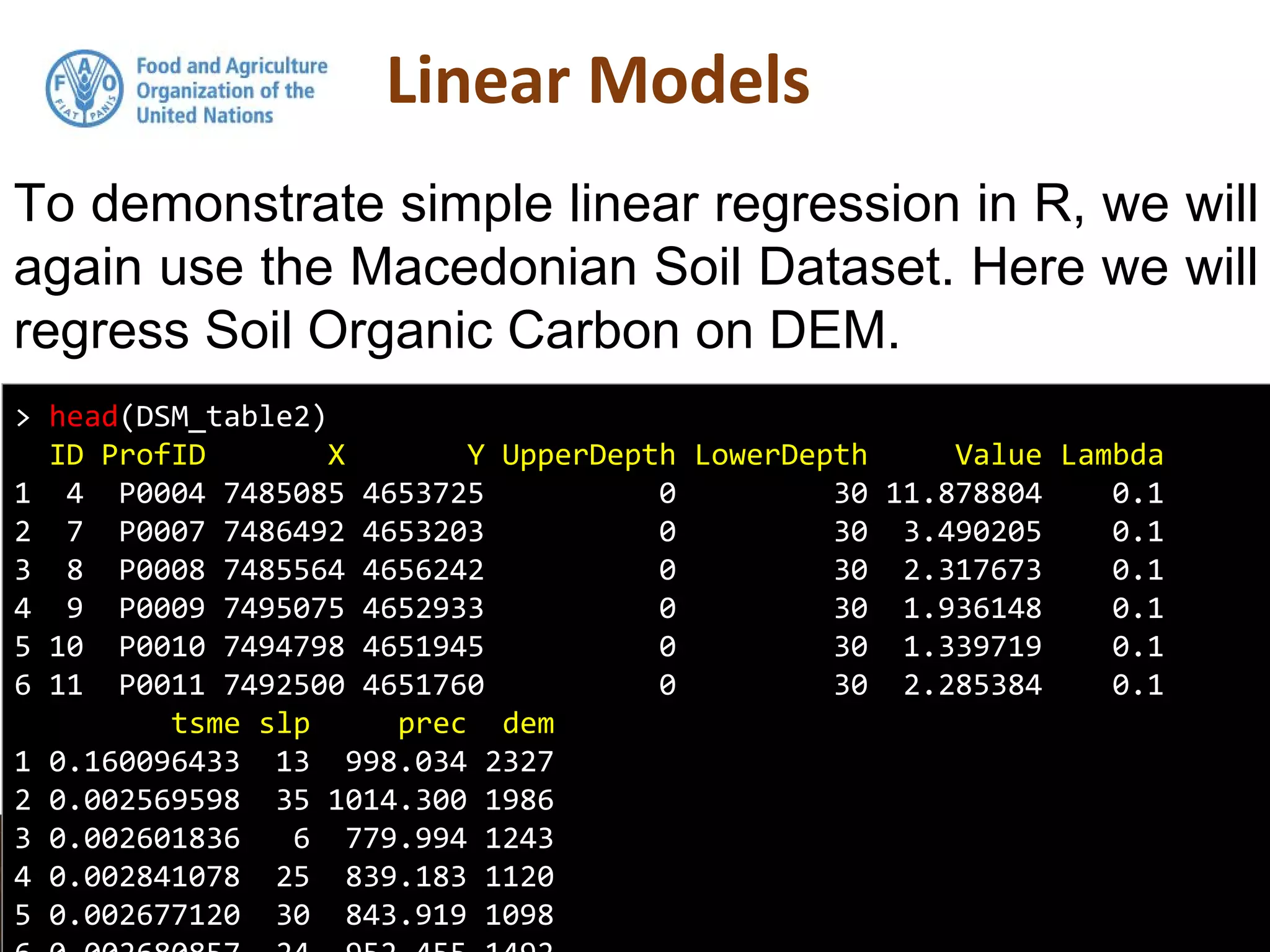
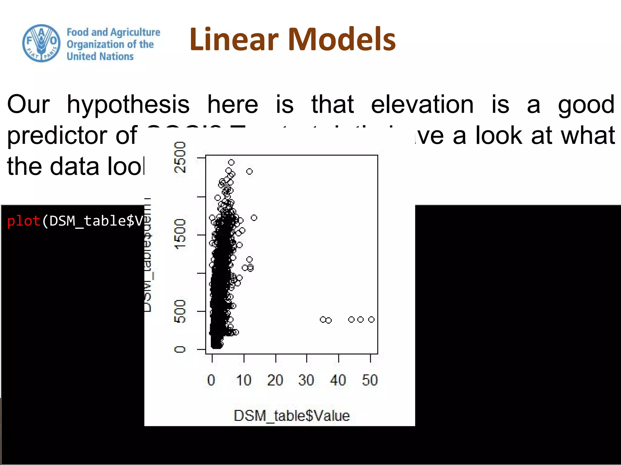
Simple linear regression uses a single independent variable to predict the value of a dependent variable. Multiple linear regression extends this to use multiple independent variables to predict the dependent variable. The document demonstrates multiple linear regression in R by regressing soil organic carbon (SOC) on elevation, precipitation, and slope using the lm() function. This produces a model object that contains coefficients, residuals, fitted values and other details about the regression model.


![[1062BPY12001] Data analysis with R / week 2](https://cdn.slidesharecdn.com/ss_thumbnails/dataanalyzer01-180307063046-thumbnail.jpg?width=640&height=640&fit=bounds)


