In this work, we use genetic algorithms to combine the similarity measures so as to get the best performance. The weightage given to different similarity measures evolves over a number of generations so as to get the best combination. We test our approach on a number of benchmark time series datasets and presented promising results.

1. Combination of Similarity Measures for Time
Series Classification using Genetic Algorithms
Deepti Dohare and V. Susheela Devi
Department of Computer Science and Automation
Indian Institute of Science, India
{deeptidohare, susheela}@csa.iisc.ernet.in
Abstract—Time series classification deals with the problem
of classification of data that is multivariate in nature. This
means that one or more of the attributes is in the form of
a sequence. The notion of similarity or distance, used in time
series data, is significant and affects the accuracy, time, and
space complexity of the classification algorithm. There exist
numerous similarity measures for time series data, but each of
them has its own disadvantages. Instead of relying upon a single
similarity measure, our aim is to find the near optimal solution
to the classification problem by combining different similarity
measures. In this work, we use genetic algorithms to combine
the similarity measures so as to get the best performance. The
weightage given to different similarity measures evolves over a
number of generations so as to get the best combination. We test
our approach on a number of benchmark time series datasets
and present promising results.
I. INTRODUCTION
Time series data are ubiquitous, as most of the data is in
the form of time series, for example, stocks, annual rainfall,
blood pressure, etc. In fact, other forms of data can also be
meaningfully converted to time series including text, DNA,
video, audio, images, etc [1]. It is also evident that there has
been a strong interest in applying data mining techniques to
time series data.
The problem of classification of time series data is an
interesting problem in the field of data mining. The need to
classify time series data occurs in broad range of real-world
applications like medicine, science, finance, entertainment, and
industries. In cardiology, ECG signals (an example of time
series data) are classified in order to see whether the data
comes from a healthy person or from a patient suffering from
heart disease [2]. In anomaly detection, users’ system access
activities on Unix system are monitored to detect any kind
of abnormal behavior [3]. In information retrieval, different
documents are classified into different topic categories which
has been shown to be similar to time series classification [4].
Another example in this respect is the classification of signals
coming either from nuclear explosions or from earthquakes,
in order to monitor a nuclear test ban treaty [5].
Generally, a time series t = t1, ..., tr, is an ordered set
of r data points. Here the data points, t1, ..., tr, are typically
measured at successive point of time spaced at uniform time
intervals. A time series may also carry a class label. The
problem of time series classification is to learn a classifier
C, which is a function that maps a time series t to a class
label l, that is, C(t) = l where l ∈ L, the set of class labels.
The time series classification methods can be divided into
three large categories. The first is the distance based clas-
sification method which requires a measure to compute the
distance or similarity between pairs of time sequences [6]–[8].
The second is the feature based classification method which
transforms each time series data into a feature vector and
then applies conventional classification method [9], [10]. The
third is the model based classification methods where a model
such as Hidden Markov Model (HMM) or any other statistical
model is used to classify time series data [11], [12].
In this paper, we consider the distance based classification
method where the choice of the similarity measure affects
the accuracy, as well as the time and the space complexity
of classification algorithms [6]. There exist some similarity
measures for time series data, but each of them has their
own disadvantages. Some well known similarity measures for
time series data are Euclidean distance, Dynamic time warping
distance (DTW), Longest Common Subsequence (LCSS) etc.
We introduce a similarity based time series classification algo-
rithm that uses the concept of genetic algorithms. One nearest
neighbor (1NN) classifier has often been found to perform
better than any other method for time series classification [7].
Due to the effectiveness and the simplicity of 1NN classifier,
we focus on combining different similarity measures into one
and use the resultant similarity measure with 1NN classifier.
The paper is organized as follows: We present a brief survey
of the related work in Section II. We formally define our
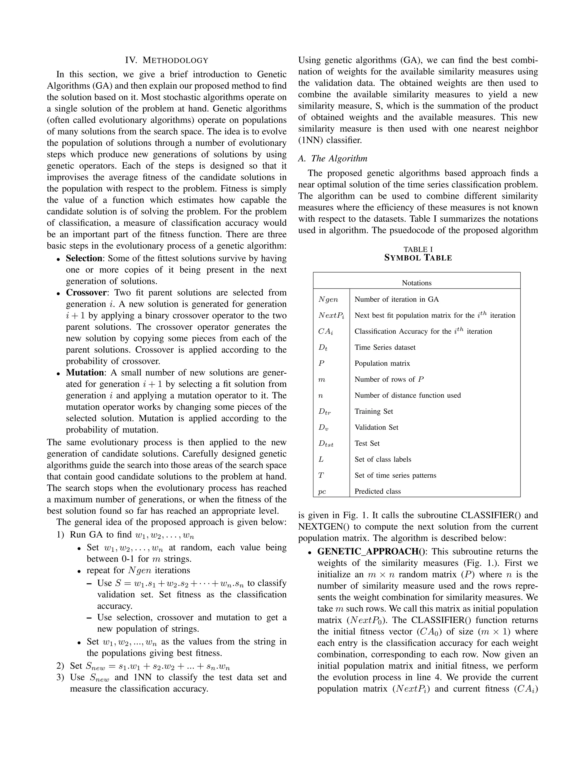
problem in Section III. In Section IV, we describe the proposed
genetic approach for the time series classification. Section V
presents the experimental evaluation. Results are shown in
Section VI. Finally, we conclude in Section VII.
II. RELATED WORK AND MOTIVATION
We begin this section with a brief description of the dis-
tance based classification method. The distance based method
requires a similarity measure or a distance function, which
is used with some existing classification algorithms. In the
current literature, there are over a dozen distance measures
for finding the similarity of time series data. Although many
algorithms have been proposed providing a new similarity
measure as a subroutine to 1NN classifier, it has been shown

2. that one nearest neighbor with Euclidean distance (1NN-ED) is
very difficult to beat [7]. However, Euclidean distance also has
some disadvantages, for instance, it is sensitivity to distortions
in time dimension. Dynamic time warping distance (DTW)
[13] is proposed to overcome this problem. It allows a time
series to be “stretched” or “compressed” to provide a better
match with another time series. DTW has been shown to be
more accurate than Euclidean distance for small datasets [8].
However, on large datasets, the accuracy of DTW converges
with Euclidean distance [6]. Due to the quadratic complexity,
DTW is costly on large datasets. Several lower bounding
measures have been introduced to speed up similarity search
using DTW [14]–[16]. Ratanamahatana and Keogh [17] pro-
posed a method that dramatically increases the speed of DTW
similarity search process by using tight lower bounds to prune
many of the calculations and it has been shown that the
amortized cost for computing DTW distance on large datasets
is linear. Xi et al. [8] use numerical reduction to speed up
DTW computation.
Another technique to describe the similarity is based on the
concept of edit distance for strings. A well known similarity
measure in this respect is the Longest Common Subsequence
(LCSS) distance [18]. The idea behind this measure is to find
the longest common subsequence of two sequences and the
distance is then defined as the length of the subsequence. A
threshold parameter ε, is used such that the two points from
different time series are considered to match if their distance
is less than ε. Another similarity measure is the Edit Distance
on Real sequence (EDR) [19] which is also based on edit
distance for strings. It also uses a threshold parameter ε but
here the distance between a pair of points is quantified to 0
or 1. EDR assigns penalties to the unmatched segments of
two time series based on the length of the segments. The Edit
Distance with Real Penalty (ERP) distance [20] is another
similarity measure that combines the merits of DTW and EDR.
ERP computes the distance between gaps of two time series
by using a constant reference point. If the distance between
the two points is large, ERP selects the distance between
the reference point and one of those points. Lee et al. [21]
point out that the disadvantage of the above distance measures
(LCSS, EDR, ERP) is that these measures capture the global
similarity between two sequences, but not their local similarity
during a short time interval. Other distance measures are:
DISSIM [22], Sequence Weighted Alignment model (Swale)
[23], Spatial Assembling Distance (SpADe) [24] and similarity
search based on Threshold Queries (TQuEST) [25] etc.
A. Motivation
Although, most of the newly introduced similarity measures
have been shown to perform well, each of them has its own
disadvantages. Also, the efficiency of a similarity measure
depends critically on the size of the dataset [6]. So, instead
of deciding which is the single best performing similarity
measure for the classification task on a dataset, we make use of
a number of distance measures and appropriately weigh their
performance with the help of some kind of heuristic. Motivated
by these considerations, we combine different existing similar-
ity measures to find near-optimal solutions using a stochastic
technique. We make use of Genetic Algorithms [26], [27] ,
which are popular stochastic algorithms for estimating near-
optimal solutions. Although, there is a vast amount of literature
on time series classification and mining, we believe that we are
solving the problem in a novel way. The closest work is that
of [28]. Here, the authors make use an ensemble of multiple
kNN classifiers based on different distance functions for text
classification, whereas we are applying genetic algorithms
to combine different similarity measures to achieve a better
classification accuracy. Another difference is that we are doing
this for time series data where finding a good similarity
measure is non trivial.
III. PROBLEM DEFINITION
We will now define our problem formally. A time series
t = [t1, t2, . . . , tr]
where t1, t2, . . . , tr are the data points, measured at uniform
time intervals. T is the set of such time series. Let Dtr be a
training set represented as a matrix of size, q × r,
Dtr = [tr1, tr2, . . . , trq]T
where tri ∈ T. In this work, we consider labeled time series
where Ltr is a vector of class labels of training set Dtr,
Ltr = [l1, l2, . . . , lq]T
where li ∈ L, L is the set of class labels. The test set is a
matrix of size, p × r,
Dtst = [ts1, ts2, . . . , tsp]T
where tsi ∈ T.
Input: A time series dataset partitioned into the training set
Dtr with class labels Ltr, and the test set Dtst
Output: A classifier C such that C(t) = l where l ∈ L and
t ∈ T.
The problem of time series classification is to learn a
classifier C, which is a function C : T → L. Here, we are
not designing a classifier, we are using 1NN classifier which
requires a similarity measure for time series classification. As
mentioned in Section II, there are different similarity measures,
but we might not know which similarity measure is best suited
for the dataset. Our aim in this work is to combine different
similarity measures (s1, s2, . . . , sn) by assigning them some
weight based on their performance. A new similarity measure
(Snew) is obtained such that
Snew =
n
i=1
wi · si
where r is the number of similarity measures. The parameter
of evaluating the solution in our approach is the accuracy.

3. IV. METHODOLOGY
In this section, we give a brief introduction to Genetic
Algorithms (GA) and then explain our proposed method to find
the solution based on it. Most stochastic algorithms operate on
a single solution of the problem at hand. Genetic algorithms
(often called evolutionary algorithms) operate on populations
of many solutions from the search space. The idea is to evolve
the population of solutions through a number of evolutionary
steps which produce new generations of solutions by using
genetic operators. Each of the steps is designed so that it
improvises the average fitness of the candidate solutions in
the population with respect to the problem. Fitness is simply
the value of a function which estimates how capable the
candidate solution is of solving the problem. For the problem
of classification, a measure of classification accuracy would
be an important part of the fitness function. There are three
basic steps in the evolutionary process of a genetic algorithm:
• Selection: Some of the fittest solutions survive by having
one or more copies of it being present in the next
generation of solutions.
• Crossover: Two fit parent solutions are selected from
generation i. A new solution is generated for generation
i + 1 by applying a binary crossover operator to the two
parent solutions. The crossover operator generates the
new solution by copying some pieces from each of the
parent solutions. Crossover is applied according to the
probability of crossover.
• Mutation: A small number of new solutions are gener-
ated for generation i + 1 by selecting a fit solution from
generation i and applying a mutation operator to it. The
mutation operator works by changing some pieces of the
selected solution. Mutation is applied according to the
probability of mutation.
The same evolutionary process is then applied to the new
generation of candidate solutions. Carefully designed genetic
algorithms guide the search into those areas of the search space
that contain good candidate solutions to the problem at hand.
The search stops when the evolutionary process has reached
a maximum number of generations, or when the fitness of the
best solution found so far has reached an appropriate level.
The general idea of the proposed approach is given below:
1) Run GA to find w1, w2, . . . , wn
• Set w1, w2, . . . , wn at random, each value being
between 0-1 for m strings.
• repeat for Ngen iterations
– Use S = w1.s1 +w2.s2 +· · ·+wn.sn to classify
validation set. Set fitness as the classification
accuracy.
– Use selection, crossover and mutation to get a
new population of strings.
• Set w1, w2, ..., wn as the values from the string in
the populations giving best fitness.
2) Set Snew = s1.w1 + s2.w2 + ... + sn.wn
3) Use Snew and 1NN to classify the test data set and
measure the classification accuracy.
Using genetic algorithms (GA), we can find the best combi-
nation of weights for the available similarity measures using
the validation data. The obtained weights are then used to
combine the available similarity measures to yield a new
similarity measure, S, which is the summation of the product
of obtained weights and the available measures. This new
similarity measure is then used with one nearest neighbor
(1NN) classifier.
A. The Algorithm
The proposed genetic algorithms based approach finds a
near optimal solution of the time series classification problem.
The algorithm can be used to combine different similarity
measures where the efficiency of these measures is not known
with respect to the datasets. Table I summarizes the notations
used in algorithm. The psuedocode of the proposed algorithm
TABLE I
SYMBOL TABLE
Notations
Ngen Number of iteration in GA
NextPi Next best fit population matrix for the ith iteration
CAi Classification Accuracy for the ith iteration
Dt Time Series dataset
P Population matrix
m Number of rows of P
n Number of distance function used
Dtr Training Set
Dv Validation Set
Dtst Test Set
L Set of class labels
T Set of time series patterns
pc Predicted class
is given in Fig. 1. It calls the subroutine CLASSIFIER() and
NEXTGEN() to compute the next solution from the current
population matrix. The algorithm is described below:
• GENETIC APPROACH(): This subroutine returns the
weights of the similarity measures (Fig. 1.). First we
initialize an m × n random matrix (P) where n is the
number of similarity measure used and the rows repre-
sents the weight combination for similarity measures. We
take m such rows. We call this matrix as initial population
matrix (NextP0). The CLASSIFIER() function returns
the initial fitness vector (CA0) of size (m × 1) where
each entry is the classification accuracy for each weight
combination, corresponding to each row. Now given an
initial population matrix and initial fitness, we perform
the evolution process in line 4. We provide the current
population matrix (NextPi) and current fitness (CAi)

4. to the function NEXTGEN() which returns the next
population matrix (NextPi+1) and next fitness vector
(CAi+1). The evolution process is run for Ngen times.
At the end of the algorithm, the genetic approach will
return the best combination of weights with maximum
fitness.
GENETIC APPROACH(Ngen, m, n)
1: Initialize an m × n P matrix where each element is
randomly generated
2: CA0 ← CLASSIFIER(P)
3: NextP0 ← P
4: for i ← 1 to Ngen do
5: CAi,NextPi ←NEXTGEN(CAi−1,NextPi−1)
6: end for
7: return weights with maximum fitness
Fig. 1. Finding the best weight combination of various
similarity measures using GA.
• CLASSIFIER(): The accuracy on the validation set for
all the rows of P is calculated as shown in Fig. 2. It
predicts the class label of each validation time series
object by using the combined similarity measure (line
10). Note that, the combined similarity measure in line
8 is obtained by multiplying the elements of P with
similarities of validation and training object resulting
from different distance functions. Finally, this subroutine
returns the classification accuracy for all the rows of P.
• NEXTGEN(): The main aim of this subroutine is to apply
the genetic operators, selection, crossover and mutation
on the current population matrix NextPi based on current
fitness vector CAi to yield the next population matrix
(NextPi+1). The CLASSIFIER() subroutine is called
again to get the next fitness vector (CAi+1). This function
returns the next fitness and next population matrix.
V. EXPERIMENTAL EVALUATION
We tested our proposed genetic algorithms based approach
on various benchmark datasets from the UCR classifica-
tion/clustering archive [29]. Table II shows the statistics of
the datasets used in our experiment.
A. Procedure
• We divide the original training set of the benchmark
datasets into two sets: the training set and the validation
set.
• The training set and the validation set is then provided
to the proposed GENETIC APPROACH which gives the
best combination of weights (w1, w2, . . . , wn) for the n
similarity measures.
• The resultant weights are assigned to the different sim-
ilarity measures which are combined to yield the new
CLASSIFIER(P)
1: for i ← 1 to m do
2: for j ← 1 to size(Dv) do
3: best so far ← inf
4: for k ← 1 to size(Dtr) do
5: x←training pattern
6: y←Validation pattern
7: Compute s1, s2, ..., sn distance function for x
and y
8: S[i] ← s1∗P[i][1]+s2∗P[i][2]+....+sn∗P[i][n]
9: if S[i] < best so far then
10: pc ← Train Class labels[k]
11: end if
12: end for
13: if predicted class (pc) is same as the actual class
then
14: correct ← correct + 1
15: end if
16: end for
17: CA ← (correct/size(Dv)) ∗ 100
18: end for
19: return CA
Fig. 2. Subroutine CLASSIFIER: Computation of CA for
one population matrix P of size m × n .
NEXTGEN(CA, P)
1: P ← P
2: fitness ← CA
3: Generate P from P by applying selection
{Selection}
4: Generate P from P by applying crossover
{Crossover}
5: Select randomly some elements of P and change the
values.
{Mutation}
6: NextP ← P
7: NextCA ←CLASSIFIER(P)
8: return NextCA, NextP
Fig. 3. Subroutine NEXTGEN: Applying Genetic Opera-
tors (selection, crossover and mutation) to produce next
population matrix NextP .
similarity measure which is:
Snew = s1.w1 + s2.w2 + · · · + sn.wn
• This new similarity measure Snew is then used to classify
the test data using 1NN which gives the final classifica-
tion accuracy.

5. TABLE II
STATISTICS OF THE DATASETS USED IN OUR
EXPERIMENT
Number Size of Size of Size of Time
Dataset of training validation test series
classes set set set Length
Control Chart 6 180 120 300 60
Coffee 2 18 10 28 286
Beef 5 18 12 30 470
OliveOil 4 18 12 30 570
Lightning-2 2 40 20 61 637
Lightning-7 7 43 27 73 319
Trace 4 62 38 100 275
ECG 2 67 33 100 96
B. Similarity Measures
In order to test the genetic approach empirically, we im-
plemented the algorithm using eight distance functions. Given
two time series:
p = (p1, p2, ..., pn)
q = (q1, q2, ..., qn)
a similarity function s calculates the distance between the two
time series, denoted by s(p, q). The eight similarity measures
used in implementation are:
1) Euclidean Distance (L2 norm): For simple time series
classification, Euclidean distance is a widely adopted
option. The distance from p to q is given by:
s1(p, q) =
n
i=1
(pi − qi)2
2) Manhattan Distance (L1 norm): The distance function
is given by:
s2(p, q) =
n
i=1
|(pi − qi)|
3) Maximum Norm (L∞ norm): The infinity norm dis-
tance is also called Chebyshev distance. The distance
function is given by:
s3(p, q) = max(|(p1 − q1)|, |(p2 − q2)|, ..., |(pn − qn)|)
4) Mean dissimilarity: Fink and Pratt [30] proposed a
similarity measure between two numbers a and b as :
sim(a, b) = 1 −
|a − b|
|a| + |b|
They define two similarities, mean similarity and root
mean square similarity. We use the above similarity
measure to define a distance function:
disim(a, b) =
|a − b|
|a| + |b|
and then define Mean dissimilarity as:
s4(p, q) =
1
n
.
n
i=1
disim(pi, qi)
where
disim(pi, qi) =
|pi − qi|
|pi| + |qi|
5) Root Mean Square Dissimilarity: By using the above
similarity measure, we define Root Mean Square Dis-
similarity as:
s5(p, q) =
1
n
.
n
i=1
dissim(pi, qi)2
6) Peak Dissimilarity: In addition to above similarity
measures, Fink and Pratt [30] also define peak similarity
between two numbers a and b as:
psim(a, b) = 1 −
|a − b|
2.max(|a|, |b|)
and then define peak dissimilarity as
peakdisim(pi, qi) =
|pi − qi|
2.max(|pi|, |qi|)
The peak dissimilarity between two time series p and q
is given by:
s6(p, q) =
1
n
.
n
i=1
peakdisim(pi, qi)
7) Cosine Distance: Cosine similarity is a measure of
similarity between two vectors of n dimensions by
finding the cosine of the angle between them. Given
two time series p and q, the cosine similarity, θ, is
represented using a dot product and magnitude as:
cos(θ) =
p.q
p q
and cosine dissimilarity as:
s7(p, q) = 1 − cos(θ)
8) Dynamic Time Warping Distance: In order to calculate
DTW(p, q) [17], we create a matrix of size |p| × |q|
where each element is the squared distance, d(pi, qj) =
(pi − qj)2
, between every pair of point in two time
series. Every possible warping between two time series,
is a path W, though the matrix. A warping path W, is
a contiguous set of matrix elements that characterizes
a mapping between p and q where kth
element of W

6. is defined as wk = (i, j)k. We want the best path that
minimizes the warping cost:
s8(p, q) = DTW(p, q) = min
K
k=1
wk/K
where max(|p|, |q|)≤ K < |p| + |q| − 1. This path
can be found using dynamic programming to evaluate
the following recurrence which defines the cumulative
distance γ(i, j). The recursive function γ(i, j) gives us
the minimum cost path:
γ(i, j) = d(pi, qj) + min{γ(i − 1, j − 1),
γ(i − 1, j),
γ(i, j − 1)}
C. Experiments Conducted
We initialize a 10 × 10 population matrix, P, where each
entry represents weights with random values between 0 to 1.
The function CLASSIFIER() combines the above similarity
measures to yield the resultant measure which is
Si = s1.P(i, 1) + s2.P(i, 2) + .... + sn.P(i, n)
for ith
row of P. We run the evolution process of genetic
algorithm for ten iterations (Ngen = 10) and the solution
obtained in every generation is used to generate the next better
solution. We used deterministic selection and single point
crossover in the NEXTGEN() function. After ten iterations,
the GENETIC APPROACH() returns the best combination
of weights for the tenth generation. The weights are then
combined to yield a new similarity measure. This similarity
measure is then used to classify the test data Dtst of the dataset
Dt. Note that, one may use many other similarity measures
also as candidate distance measures, for example, elastic
measures (ERP, EDR, LCSS etc), threshold based measures
(eg. TQuEST) or pattern based measures (eg. SpADe) instead
of any of the measure that we have used.
VI. RESULTS
In this section, we will elaborately describe the results.
Table III shows the weights obtained after ten iterations for the
eight benchmark datasets using the validation set. We can see
from the table that the highest weight is assigned to the most
efficient similarity measure. The inefficient similarity measure
with respect to others, are simply discarded as the weights
assigned to them is zero or negligible. For example, for the
Control Chart dataset, the weight assigned to DTW (s8) is
more than that of Euclidean distance (s1) whereas for the
Lighting2 dataset, weight assigned to Euclidean distance is
more than the weight given to DTW. Note that, the Maximum
Norm (L∞ norm) distance function, which is considered
inefficient as compared to Euclidean Distance and DTW, has
highest weight in case of Coffee dataset. We do not have
to pre-specify a distance measure for a particular dataset, as
TABLE III
WEIGHTS ASSIGNED TO EACH SIMILARITY MEASURE
AFTER 10 ITERATIONS.
Dataset s1 s2 s3 s4 s5 s6 s7 s8
Control Chart 0.72 0.29 0.33 0.18 0.12 0.61 0.31 0.82
Coffee 0.74 0.9 0.9 0.1 0.03 0.03 0.06 0.70
Beef 0.95 0.09 0 0.48 0 0.62 0.58 0.73
OliveOil 0.7 0 0.79 0 0 0 0.58 0.67
Lightning-2 0.99 0.75 0.79 0.09 0.21 0.09 0.71 0.97
Lightning-7 0.95 .06 0.09 0.81 0.95 0.29 0.38 0.99
Trace 0.62 0.08 0.28 0.39 0.14 0.47 0.23 0.98
ECG 0.052 0 0.21 0 0 0.98 0.90 0
we might not know what kind of similarities exist in the
data. Instead of depending on a single similarity measure
beforehand, we find a weighted combination of different
similarity measures for the classification task. This is the main
advantage of combining similarity measures. Thus, Genetic
Algorithms guide us in estimating near-optimal solutions of
the time series classification problem.
We find the accuracy with each of the eight similarity mea-
sures using one nearest neighbour classifier on all the datasets.
Fig. 4. shows the classification accuracy for each similarity
measure. The weighted combination of the eight similarity
measures is used with one nearest neighbour classifier to
classify the test set of the benchmark datasets.
The results are shown in Table IV. It compares the results
obtained from the proposed genetic approach, with 1NN-ED,
1NN-DTW and other classifier based on similarity measures
given in Section V. In most cases, the classification accuracy
obtained from our approach by using the weighted combina-
tion of similarity measures, exceeds the classification accuracy
obtained using individual similarity measures. Even though, in
many cases, the accuracy obtained by 1NN-DTW matches the
accuracy obtained with our approach, in some cases like ECG
and Coffee, our method gives significantly better results.
VII. CONCLUSION
We presented a novel algorithm for time series classification
using the combination of different similarity measures based
on Genetic Algorithms. Since different similarity measure are
put together, we obtain large number of solution sets. The
advantage of using genetic algorithm is that an inefficient
similarity measure does not affect the proposed algorithm as it
will be simply discarded in next generated solution. Thus, we
can say that the genetic algorithms based approach, proposed
by us, is guaranteed to yield better results. Although, obtaining
the combination of similarity measures may take time, but it

7. Fig. 4. Classification Accuracy for different similarity measures on various datasets from the UCR classification/clustering
archive [29]
TABLE IV
COMPARISON OF CLASSIFICATION ACCURACY USING OUR SIMILARITY MEASURE AND OTHER SIMILARITY
MEASURES.
Dataset Size (using our (1NN-ED) (1NN-L1) (1NN-L∞ (1NN- (1NN- (1NN- (1NN- (Traditional
approach) norm) norm) disim) rootdisim) peakdisim) cosine) 1NN-DTW)
Control Chart 600 99.33% 88% 88% 81.33% 58% 53% 77% 80.67% 99.33%
Coffee 56 89.28% 75% 79.28% 89.28% 75% 75% 75% 53.57% 82.14%
Beef 60 53.34% 53.33% 50% 53.33% 46.67% 50% 46.67% 20% 50%
OliveOil 121 86.67% 86.67% 36.67% 83.33% 63.33% 60% 63.33% 16.67% 86.67%
Lightning-2 121 86.89% 74.2% 52.4% 68.85% 55.75% 50.81% 83.60% 63.93% 85.25%
Lightning-7 143 67.12% 67.53% 24.65% 45.21% 34.24% 28.76% 61.64% 53.42% 72.6%
Trace 200 100% 76% 74% 69% 65% 57% 75% 53% 100%
ECG 200 91% 88% 66% 87% 79% 79% 91% 81% 77%
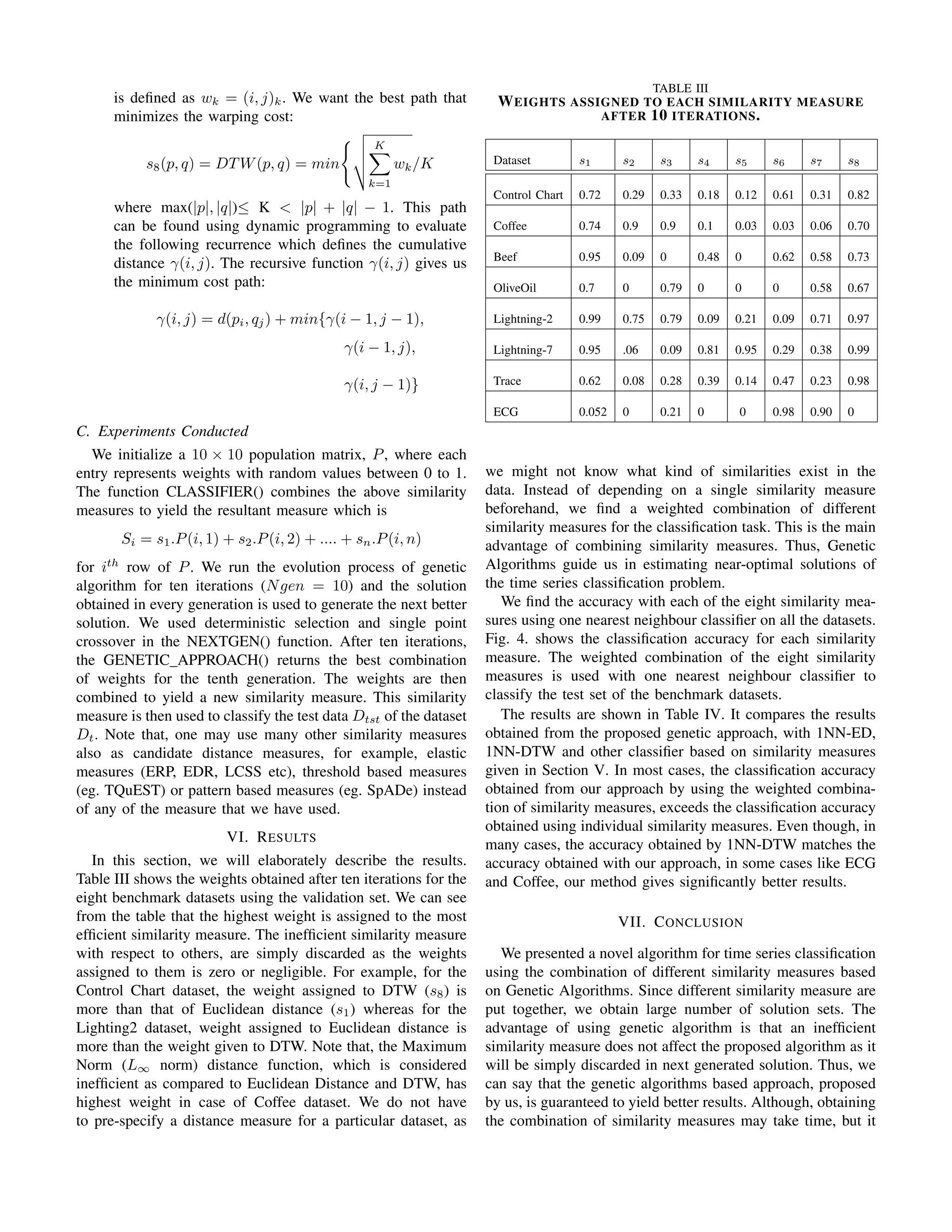
is only the design time. Once the combination is obtained, it
can be easily used for classifying new patterns.
The implementation of the proposed algorithm has shown
that the results obtained using this approach are considerably
better.
The future work can be extended in the following directions:
• It would be interesting to see whether our approach can
be applied to various other kinds of datasets with little or
no modification, for example, streaming datasets.
• The algorithm can be used with any distance based
classifier. We wish to present results by using other
classifiers.
• Other similarity measures can also be used in the pro-
posed genetic algorithm based approach.
REFERENCES
[1] E. Keogh, “Recent advances in mining time series data,” in Knowledge
Discovery in Databases: PKDD 2005, ser. Lecture Notes in Computer
Science, A. Jorge, L. Torgo, P. Brazdil, R. Camacho, and J. Gama, Eds.
Springer Berlin / Heidelberg, 2005, vol. 3721, pp. 6–6.
[2] L. Wei and E. Keogh, “Semi-supervised time series classification,” in
Proceedings of the 12th ACM SIGKDD international conference on
Knowledge discovery and data mining, ser. KDD ’06. New York,
NY, USA: ACM, 2006, pp. 748–753.
[3] T. Lane and C. E. Brodley, “Temporal sequence learning and data
reduction for anomaly detection,” ACM Trans. Inf. Syst. Secur., vol. 2,
pp. 295–331, August 1999.
[4] F. Sebastiani, “Machine learning in automated text categorization,” ACM
Comput. Surv., vol. 34, pp. 1–47, March 2002.
[5] R. H. S. Y. Kakizawa and M. Taniguchi, “Discrimination and clustering
for multivariate time series.” Journal of the American Statistical Asso-
ciation, vol. 93, pp. 328–340, 1998.
[6] H. Ding, G. Trajcevski, P. Scheuermann, X. Wang, and E. Keogh,
“Querying and mining of time series data: experimental comparison of
representations and distance measures,” Proc. VLDB Endow., vol. 1, pp.
1542–1552, August 2008.
[7] E. Keogh and S. Kasetty, “On the need for time series data mining
benchmarks: A survey and empirical demonstration,” in SIGKDD’02,
2002, pp. 102–111.
[8] X. Xi, E. Keogh, C. Shelton, L. Wei, and C. A. Ratanamahatana, “Fast
time series classification using numerosity reduction,” in ICML06, 2006,
pp. 1033–1040.
[9] N. Lesh, M. J. Zaki, and M. Ogihara, “Mining features for sequence
classification,” in Proceedings of the fifth ACM SIGKDD international
conference on Knowledge discovery and data mining, ser. KDD ’99.
New York, NY, USA: ACM, 1999, pp. 342–346.

8. [10] N. A. Chuzhanova, A. J. Jones, and S. Margetts, “Feature selection for
genetic sequence classification.” Bioinformatics, vol. 14, no. 2, pp. 139–
143, 1998.
[11] O. Yakhnenko, A. Silvescu, and V. Honavar, “Discriminatively trained
markov model for sequence classification,” in Proceedings of the Fifth
IEEE International Conference on Data Mining, ser. ICDM ’05. Wash-
ington, DC, USA: IEEE Computer Society, 2005, pp. 498–505.
[12] D. D. Lewis, “Naive (bayes) at forty: The independence assumption in
information retrieval,” in Proceedings of the 10th European Conference
on Machine Learning. London, UK: Springer-Verlag, 1998, pp. 4–15.
[13] E. J. Keogh and M. J. Pazzani, “Scaling up dynamic time warping
for datamining applications,” in Proceedings of the 6th Int. Conf. on
Knowledge Discovery and Data Mining, 2000, pp. 285–289.
[14] E. Keogh, “Exact indexing of dynamic time warping,” in Proceedings of
the 28th international conference on Very Large Data Bases, ser. VLDB
’02. VLDB Endowment, 2002, pp. 406–417.
[15] E. Keogh and C. A. Ratanamahatana, “Exact indexing of dynamic time
warping,” Knowl. Inf. Syst., vol. 7, pp. 358–386, March 2005.
[16] S.-W. Kim, S. Park, and W. Chu, “An index-based approach for similarity
search supporting time warping in large sequence databases,” in Data
Engineering, 2001. Proceedings. 17th International Conference on,
2001, pp. 607 –614.
[17] C. A. Ratanamahatana and E. Keogh, “Making time-series classification
more accurate using learned constraints,” in SDM 04: SIAM Interna-
tional Conference on Data Mining, 2008.
[18] D. Gunopulos, G. Kollios, and M. Vlachos, “Discovering similar mul-
tidimensional trajectories,” in 18th International Conference on Data
Engineering, 2002, pp. 673–684.
[19] L. Chen, M. T. ¨Ozsu, and V. Oria, “Robust and fast similarity search for
moving object trajectories,” in Proceedings of the 2005 ACM SIGMOD
international conference on Management of data, ser. SIGMOD ’05.
New York, NY, USA: ACM, 2005, pp. 491–502.
[20] L. Chen and R. Ng, “On the marriage of lp-norms and edit distance,”
in Proceedings of the Thirtieth international conference on Very large
data bases - Volume 30, ser. VLDB ’04. VLDB Endowment, 2004,
pp. 792–803.
[21] J.-G. Lee, J. Han, and K.-Y. Whang, “Trajectory clustering: a partition-
and-group framework,” in Proceedings of the 2007 ACM SIGMOD
international conference on Management of data, ser. SIGMOD ’07.
New York, NY, USA: ACM, 2007, pp. 593–604.
[22] E. Frentzos, K. Gratsias, Y. Theodoridis, E. Frentzos, K. Gratsias, and
Y. Theodoridis, “Index-based most similar trajectory search,” 2006.
[23] M. D. Morse and J. M. Patel, “An efficient and accurate method for
evaluating time series similarity,” in Proceedings of the 2007 ACM SIG-
MOD international conference on Management of data, ser. SIGMOD
’07, New York, NY, USA, 2007, pp. 569–580.
[24] Y. Chen, M. A. Nascimento, B. C. Ooi, and A. K. H. Tung, “Spade: On
shape-based pattern detection in streaming time series,” Data Engineer-
ing, International Conference on, vol. 0, pp. 786–795, 2007.
[25] J. Afalg, H.-P. Kriegel, P. Krger, P. Kunath, A. Pryakhin, and M. Renz,
“Similarity search on time series based on threshold queries,” in Ad-
vances in Database Technology - EDBT 2006, ser. Lecture Notes in
Computer Science. Springer Berlin / Heidelberg, 2006, vol. 3896, pp.
276–294.
[26] D. E. Goldberg, Genetic Algorithms in Search, Optimization and Ma-
chine Learning, 1st ed. Boston, MA, USA: Addison-Wesley Longman
Publishing Co., Inc., 1989.
[27] S. M. Thede, “An introduction to genetic algorithms,” J. Comput. Small
Coll., vol. 20, pp. 115–123, October 2004.
[28] T. Yamada, K. Yamashita, N. Ishii, and K. Iwata, “Text classification
by combining different distance functions with weights,” Software
Engineering, Artificial Intelligence, Networking and Parallel/Distributed
Computing, International Conference on and Self-Assembling Wireless
Networks, International Workshop on, vol. 0, pp. 85–90, 2006.
[29] E. Keogh, X. Xi, L. Wei, and C. A. Ratanamahatana,
The UCR Time Series Classification/Clustering Homepage,
http://www.cs.ucr.edu/∼eamonn/time series data/, 2006.
[30] E. Fink and K. B. Pratt, “Indexing of compressed time series,” in Data
Mining in Time Series Databases. World Scientific, 2004, pp. 51–78.