Download to read offline
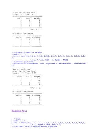
![> maxFlowFordFulkerson(nodes, arcs, source.node = 2, sink.node = 6)
$s.cut
[1] 2 3 1 5
$t.cut
[1] 4 6
$max.flow
[1] 6](https://image.slidesharecdn.com/optreespackageinr-170603195931/85/optrees-package-in-R-and-examples-optrees-finds-optimal-trees-in-weighted-graphs-4-320.jpg)

The Optrees package in R provides tools for solving optimal tree problems in weighted graphs, such as minimum cost spanning trees, minimum cost arborescences, shortest path trees, and maximum flow calculations. Examples demonstrate the use of various algorithms like Prim, Kruskal, and Dijkstra for obtaining minimum spanning trees and shortest path trees. Additionally, the package supports negative weight graphs and maximum flow calculations using the Ford-Fulkerson algorithm.