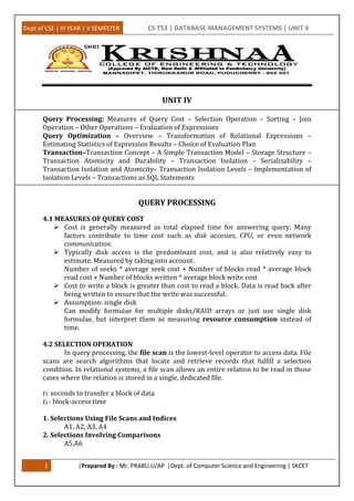
SlideShare a Scribd company logo
Dept of CSE | III YEAR | V SEMESTER CS T53 | DATABASE MANAGEMENT SYSTEMS | UNIT 4
1 |Prepared By : Mr. PRABU.U/AP |Dept. of Computer Science and Engineering | SKCET
UNIT IV
Query Processing: Measures of Query Cost – Selection Operation – Sorting – Join
Operation – Other Operations – Evaluation of Expressions
Query Optimization – Overview – Transformation of Relational Expressions –
Estimating Statistics of Expression Results – Choice of Evaluation Plan
Transaction–Transaction Concept – A Simple Transaction Model – Storage Structure –
Transaction Atomicity and Durability – Transaction Isolation – Serializability –
Transaction Isolation and Atomicity– Transaction Isolation Levels – Implementation of
Isolation Levels – Transactions as SQL Statements
QUERY PROCESSING
4.1 MEASURES OF QUERY COST
 Cost is generally measured as total elapsed time for answering query. Many
factors contribute to time cost such as disk accesses, CPU, or even network
communication.
 Typically disk access is the predominant cost, and is also relatively easy to
estimate. Measured by taking into account.
Number of seeks * average seek cost + Number of blocks read * average block
read cost + Number of blocks written * average block write cost
 Cost to write a block is greater than cost to read a block. Data is read back after
being written to ensure that the write was successful.
 Assumption: single disk
Can modify formulae for multiple disks/RAID arrays or just use single disk
formulae, but interpret them as measuring resource consumption instead of
time.
4.2 SELECTION OPERATION
In query processing, the file scan is the lowest-level operator to access data. File
scans are search algorithms that locate and retrieve records that fulfill a selection
condition. In relational systems, a file scan allows an entire relation to be read in those
cases where the relation is stored in a single, dedicated file.
tT -seconds to transfer a block of data
tS - block-access time
1. Selections Using File Scans and Indices
A1, A2, A3, A4
2. Selections Involving Comparisons
A5,A6
Dept of CSE | III YEAR | V SEMESTER CS T53 | DATABASE MANAGEMENT SYSTEMS | UNIT 4
2 |Prepared By : Mr. PRABU.U/AP |Dept. of Computer Science and Engineering | SKCET
3. Implementation of Complex Selections
Conjunction: A conjunctive selection is a selection of the form:
Disjunction: A disjunctive selection is a selection of the form:
A disjunctive condition is satisfied by the union of all records satisfying the
individual, simple conditions
Negation: The result of a selection is the set of tuples of r for which the
condition evaluates to false. In the absence of nulls, this set is simply the set of tuples
in r that are not in
A7 (conjunctive selection using one index)
 Select a combination of i and algorithms A1 through A6 that results in the least
cost for i (r).
 Test other conditions on tuple after fetching it into memory buffer.
Dept of CSE | III YEAR | V SEMESTER CS T53 | DATABASE MANAGEMENT SYSTEMS | UNIT 4
3 |Prepared By : Mr. PRABU.U/AP |Dept. of Computer Science and Engineering | SKCET
A8 (conjunctive selection using composite index)
 An appropriate composite index (that is, an index on multiple attributes) may be
available for some conjunctive selections.
 If the selection specifies an equality condition on two or more attributes, and a
composite index exists on these combined attribute fields, then the index can be
searched directly.
 The type of index determines which of algorithms A2, A3, or A4 will be used.
A9 (conjunctive selection by intersection of identifiers)
 Another alternative for implementing conjunctive selection operations involves
the use of record pointers or record identifiers.
 This algorithm requires indices with record pointers, on the fields involved in the
individual conditions.
 The algorithm scans each index for pointers to tuples that satisfy an individual
condition.
A10 (disjunctive selection by union of identifiers)
 If access paths are available on all the conditions of a disjunctive selection, each
index is scanned for pointers to tuples that satisfy the individual condition.
 The union of all the retrieved pointers yields the set of pointers to all tuples that
satisfy the disjunctive condition.
4.3 SORTING
 We may build an index on the relation, and then use the index to read the
relation in sorted order.
 May lead to one disk block access for each tuple.
 For relations that fit in memory, techniques like quick sort can be used.
 For relations that don’t fit in memory, external sort merge is a good choice.
4.3.1 External Sort-Merge Algorithm
 Sorting of relations that do not fit in memory is called external sorting.
 The most commonly used technique for external sorting is the external sort–
merge algorithm.
 Let M denote the number of blocks in the main-memory buffer available for
sorting, that is, the number of disk blocks whose contents can be buffered in
available main memory.
1. In the first stage, a number of sorted runs are created; each run is sorted, but
contains only some of the records of the relation.
i = 0;
repeat
read M blocks of the relation, or the rest of the relation,
whichever is smaller;
sort the in-memory part of the relation;
write the sorted data to run file Ri ;
i = i + 1;
until the end of the relation
Dept of CSE | III YEAR | V SEMESTER CS T53 | DATABASE MANAGEMENT SYSTEMS | UNIT 4
4 |Prepared By : Mr. PRABU.U/AP |Dept. of Computer Science and Engineering | SKCET
2. In the second stage, the runs are merged. Suppose, for now, that the total number of
runs N is less than M, so that we can allocate one block to each run and have space left to
hold one block of output. The merge stage operates as follows:
read one block of each of the N files Ri into a buffer block in memory;
repeat
choose the first tuple (in sort order) among all buffer blocks;
write the tuple to the output, and delete it from the buffer block;
if the buffer block of any run Ri is empty and not end-of-file(Ri )
then read the next block of Ri into the buffer block;
until all input buffer blocks are empty
 The output of the merge stage is the sorted relation.
 The output file is buffered to reduce the number of disk write operations.
 The preceding merge operation is a generalization of the two-way merge used by
the standard in-memory sort– merge algorithm; it merges N runs, so it is called
an N-way merge.
Figure 4.1: External sorting using sort–merge
4.3.2 Cost Analysis of External Sort-Merge
Cost analysis:
 Total number of merge passes required: logM–1(br/M).
 Block transfers for initial run creation as well as in each pass is 2br
 for final pass, we don’t count write cost
 we ignore final write cost for all operations since the output of an
operation may be sent to the parent operation without being written to
disk.
Dept of CSE | III YEAR | V SEMESTER CS T53 | DATABASE MANAGEMENT SYSTEMS | UNIT 4
5 |Prepared By : Mr. PRABU.U/AP |Dept. of Computer Science and Engineering | SKCET
Thus total number of block transfers for external sorting:
br ( 2 logM–1(br / M)+ 1)
Cost of seeks:
 During run generation:
One seek to read each run and one seek to write each run 2 br / M
 During the merge phase:
 Buffer size: bb (read/write bb blocks at a time)
 Need 2 br / bbseeks for each merge pass
 except the final one which does not require a write
 Total number of seeks:
2 br / M+ br / bb(2 logM–1(br / M)1)
4.4 JOIN OPERATION
4.4.1 Nested-Loop Join
4.4.2 Block Nested-Loop Join
4.4.3 Indexed Nested-Loop Join
4.4.4 Merge Join
4.4.4.1 Cost Analysis
4.4.4.2 Hybrid Merge Join
4.4.5 Hash Join
4.4.5.1 Basics
4.4.5.2 Recursive Partitioning
4.4.5.3 Handling of Overflows
4.4.5.4 Cost of Hash Join
4.4.5.5 Hybrid Hash Join
4.4.6 Complex Joins
4.4.1 Nested-Loop Join
To compute the theta join
Figure 4.2: Nested-Loop Join
 Relation r is called the outer relation and relation s the inner relation of the
join, since the loop for r encloses the loop for s.
 The algorithm uses the notation tr · ts, where tr and ts are tuples; tr · ts denotes
the tuple constructed by concatenating the attribute values of tuples tr and ts
4.4.2 Block Nested-Loop Join
Block nested-loop join which is a variant of the nested-loop join where every
block of the inner relation is paired with every block of the outer relation.
Dept of CSE | III YEAR | V SEMESTER CS T53 | DATABASE MANAGEMENT SYSTEMS | UNIT 4
6 |Prepared By : Mr. PRABU.U/AP |Dept. of Computer Science and Engineering | SKCET
Figure 4.3: Blocked Nested-Loop Join
4.4.3 Indexed Nested-Loop Join
In a nested-loop join (Figure 4.2), if an index is available on the inner loop’s join
attribute, index lookups can replace file scans. For each tuple tr in the outer relation r,
the index is used to look up tuples in s that will satisfy the join condition with tuple tr.
This join method is called an indexed nested-loop join; it can be used with
existing indices, as well as with temporary indices created for the sole purpose of
evaluating the join.
4.4.4 Merge Join
 The merge-join algorithm (also called the sort-merge-join algorithm) can be
used to compute natural joins and equi-joins.
 Let r (R) and s(S) be the relations whose natural join is to be computed, and let
R ∩ S denote their common attributes.
 Suppose that both relations are sorted on the attributes R ∩ S.
 Then, their join can be computed by a process much like the merge stage in the
merge–sort algorithm.
4.4.4.1 Cost Analysis
The cost of merge join is:
br + bs block transfers + br / bb+ bs / bbseeks
+ the cost of sorting if relations are unsorted.
4.4.4.2 Hybrid Merge Join
If one relation is sorted, and the other has a secondary B+ tree index on the join
attribute
 Merge the sorted relation with the leaf entries of the B+ tree.
 Sort the result on the addresses of the unsorted relation’s tuples.
 Scan the unsorted relation in physical address order and merge with previous
result, to replace addresses by the actual tuples.
 Sequential scan more efficient than random lookup.
4.4.5 Hash Join
4.4.5.1 Basics
 The idea behind the hash-join algorithm is this: Suppose that an r tuple and an s
tuple satisfy the join condition; then, they have the same value for the join
attributes.
Dept of CSE | III YEAR | V SEMESTER CS T53 | DATABASE MANAGEMENT SYSTEMS | UNIT 4
7 |Prepared By : Mr. PRABU.U/AP |Dept. of Computer Science and Engineering | SKCET
 If that value is hashed to some value i, the r tuple has to be in ri and the s tuple in
si. Therefore, r tuples in ri need only to be compared with s tuples in si ; they do
not need to be compared with s tuples in any other partition.
4.4.5.2 Recursive Partitioning
Recursive partitioning required if number of partitions n is greater than
number of pages M of memory.
 instead of partitioning n ways, use M – 1 partitions for s
 Further partition the M – 1 partitions using a different hash function
 Use same partitioning method on r
 Rarely required: e.g., recursive partitioning not needed for relations of 1GB or
less with memory size of 2MB, with block size of 4KB.
4.4.5.3 Handling of Overflows
Hash table overflow occurs in partition si if si does not fit in memory. Reasons
could be
 Many tuples in s with same value for join attributes
 Bad hash function
Overflow resolution can be done in build phase
 Partition si is further partitioned using different hash function.
 Partition ri must be similarly partitioned.
Overflow avoidance performs partitioning carefully to avoid overflows during build
phase.
E.g. partition build relation into many partitions, then combine them.
Both approaches fail with large numbers of duplicates.
Fallback option: use block nested loops join on overflowed partitions.
4.4.5.4 Cost of Hash Join
If recursive partitioning is not required: cost of hash join is
3(br + bs) +4 * nh block transfers + 2( br / bb+ bs / bb) seeks
If recursive partitioning required:
 number of passes required for partitioning build relation
s is logM–1(bs) – 1
 best to choose the smaller relation as the build relation.
Total cost estimate is:
2(br + bs logM–1(bs) – 1+ br + bs block transfers +
2(br / bb+ bs / bb) logM–1(bs) – 1seeks
4.4.5.5 Hybrid Hash Join
Main feature of hybrid hash join:
 Keep the first partition of the build relation in memory.
 E.g. With memory size of 25 blocks, depositor can be partitioned into five
partitions, each of size 20 blocks.
Division of memory:
 The first partition occupies 20 blocks of memory
 1 block is used for input, and 1 block each for buffering the other 4 partitions.
Dept of CSE | III YEAR | V SEMESTER CS T53 | DATABASE MANAGEMENT SYSTEMS | UNIT 4
8 |Prepared By : Mr. PRABU.U/AP |Dept. of Computer Science and Engineering | SKCET
4.4.6 Complex Joins
Joins with complex join conditions, such as conjunctions and disjunctions, can be
implemented by using the efficient join techniques.
Join with a conjunctive condition:
We can compute the overall join by first computing the result of one of these
simpler joins each pair of tuples in the intermediate result consists of one
tuple from r and one from s.
A join whose condition is disjunctive can be computed in this way. Consider:
The join can be computed as the union of the records in individual joins
4.5 OTHER OPERATIONS
4.5.1 Duplicate Elimination
4.5.2 Projection
4.5.3 Set Operations
4.5.4 Outer Join
4.5.5 Aggregation
4.5.1 Duplicate Elimination
Duplicate elimination can be implemented via hashing or sorting.
 On sorting duplicates will come adjacent to each other, and all but one set of
duplicates can be deleted.
 Optimization: duplicates can be deleted during run generation as well as at
intermediate merge steps in external sort merge.
 Hashing is similar – duplicates will come into the same bucket.
4.5.2 Projection
 Perform projection on each tuple
 Followed by duplicate elimination
4.5.3 Set Operations
Set operations (, and ): can either use variant of merge join after sorting,
or variant of hash join.
E.g., Set operations using hashing:
1. Partition both relations using the same hash function
2. Process each partition i as follows.
 Using a different hashing function, build an in memory hash index on ri.
 Process si as follows
 r s:
1. Add tuples in si to the hash index if they are not already in it.
2. At end of si add the tuples in the hash index to the result.
Dept of CSE | III YEAR | V SEMESTER CS T53 | DATABASE MANAGEMENT SYSTEMS | UNIT 4
9 |Prepared By : Mr. PRABU.U/AP |Dept. of Computer Science and Engineering | SKCET
 r s:
1. output tuples in si to the result if they are already there in the hash index.
 r – s:
1. for each tuple in si, if it is there in the hash index, delete it from the index.
2. At end of si add remaining tuples in the hash index to the result.
4.5.4 Outer Join
Outer join can be computed either as
 A join followed by addition of null-padded non participating tuples.
 by modifying the join algorithms.
Modifying merge join to compute
 In , non participating tuples are those in r-R( )
 Modify merge join to compute : During merging, for every tuple tr from r
that do not match any tuple in s, output tr padded with nulls.
 Right outer join and full outer join can be computed similarly.
Modifying hash join to compute
 If r is probe relation, output non matching r tuples padded with nulls
 If r is build relation, when probing keep track of which r tuples matched s tuples.
 At end of si output non matched r tuples padded with nulls
4.5.5 Aggregation
Aggregation can be implemented in a manner similar to duplicate elimination.
Sorting or hashing can be used to bring tuples in the same group together, and then the
aggregate functions can be applied on each group.
Optimization: combine tuples in the same group during run generation and
intermediate merges, by computing partial aggregate values.
 For count, min, max, sum: keep aggregate values on tuples found so far in the
group.
 When combining partial aggregate for count, add up the aggregates.
 For avg, keep sum and count, and divide sum by count at the end.
4.6 EVALUATION OF EXPRESSIONS
4.6.1 Materialization
4.6.2 Pipelining
4.6.2.1 Implementation of Pipelining
1. Demand-driven pipeline
2. Producer-driven pipeline
4.6.3 Evaluation Algorithms for Pipelining
4.6.1 Materialization
Materialization: generate results of an expression whose inputs are relations or are
already computed, materialize (store) it on disk.
Materialized evaluation: evaluate one operation at a time, starting at the lowest level.
Use intermediate results materialized into temporary relations to evaluate next level
operations.
Dept of CSE | III YEAR | V SEMESTER CS T53 | DATABASE MANAGEMENT SYSTEMS | UNIT 4
10 |Prepared By : Mr. PRABU.U/AP |Dept. of Computer Science and Engineering | SKCET
E.g., in figure below, compute and store then compute the store its join with customer,
and finally compute the projections on customername.
Figure 4.4: Relation
4.6.2 Pipelining
 Pipelining: pass on tuples to parent operations even as an operation is being
executed.
 Pipelined evaluation : evaluate several operations simultaneously, passing the
results of one operation on to the next.
 E.g., in previous expression tree, don’t store result of
balance2500(account)
 instead, pass tuples directly to the join. Similarly, don’t store result of join, pass
tuples directly to projection.
 Much cheaper than materialization: no need to store a temporary relation
 to disk.
 Pipelining may not always be possible – e.g., sort, hash join.
 For pipelining to be effective, use evaluation algorithms that generate output
tuples even as tuples are received for inputs to the operation.
4.6.2.1 Implementation of Pipelining
Pipelines can be executed in two ways: demand driven and producer driven.
1. Demand-driven pipeline
In demand driven or lazy evaluation,
 system repeatedly requests next tuple from top level operation.
 Each operation requests next tuple from children operations as required, in
order to output its next tuple.
 In between calls, operation has to maintain “state” so it knows what to return
next.
2. Producer-driven pipeline
In producer-driven or eager pipelining
 Operators produce tuples eagerly and pass them up to their parents.
 Buffer maintained between operators, child puts tuples in buffer, parent
removes tuples from buffer.
 if buffer is full, child waits till there is space in the buffer, and then generates
more tuples.
 System schedules operations that have space in output buffer and can process
more input tuples.
Dept of CSE | III YEAR | V SEMESTER CS T53 | DATABASE MANAGEMENT SYSTEMS | UNIT 4
11 |Prepared By : Mr. PRABU.U/AP |Dept. of Computer Science and Engineering | SKCET
4.6.3 Evaluation Algorithms for Pipelining
 Some algorithms are not able to output results even as they get input tuples
 E.g. merge join, or hash join
 intermediate results written to disk and then read back
 Algorithm variants to generate (at least some) results on the fly, as input tuples
are read
 E.g. hybrid hash join generates output tuples even as probe relation tuples
in the in memory partition (partition 0) are read
 Pipelined join technique: Hybrid hash join, modified to buffer partition 0 tuples
of both relations in memory, reading them as they become available, and output
results of any matches between partition 0 tuples
 When a new r0 tuple is found, match it with existing s0 tuples, output
matches, and save it in r0.
 Symmetrically for s0 tuples.
Dept of CSE | III YEAR | V SEMESTER CS T53 | DATABASE MANAGEMENT SYSTEMS | UNIT 4
12 |Prepared By : Mr. PRABU.U/AP |Dept. of Computer Science and Engineering | SKCET
QUERY OPTIMIZATION
4.7 OVERVIEW
Alternative ways of evaluating a given query
1. Equivalent expressions
2. Different algorithms for each operation
Figure 4.5: Equivalent expressions
An evaluation plan defines exactly what algorithm is used for each operation,
and how the execution of the operations is coordinated.
 Steps in cost based query optimization
1. Generate logically equivalent expressions using equivalence rules
2. Annotate resultant expressions to get alternative query plans
3. Choose the cheapest plan based on estimated cost
 Estimation of plan cost based on:
 Statistical information about relations. Examples:
 number of tuples, number of distinct values for an attribute
 Statistics estimation for intermediate results to compute cost of complex
expressions
 Cost formulae for algorithms, computed using statistics
Figure 4.6: Evaluation Plan
Dept of CSE | III YEAR | V SEMESTER CS T53 | DATABASE MANAGEMENT SYSTEMS | UNIT 4
13 |Prepared By : Mr. PRABU.U/AP |Dept. of Computer Science and Engineering | SKCET
4.8 TRANSFORMATION OF RELATIONAL EXPRESSIONS
Two relational algebra expressions are said to be equivalent if the two
expressions generate the same set of tuples on every legal database instance.
Note: order of tuples is irrelevant
In SQL, inputs and outputs are multisets of tuples
Two expressions in the multiset version of the relational algebra are said to be
equivalent if the two expressions generate the same multiset of tuples on every legal
database instance.
An equivalence rule says that expressions of two forms are equivalent, Can
replace expression of first form by second, or vice versa.
We use θ, θ1, θ2 and so on to denote predicates, L1, L2, L3, and so on to denote
lists of attributes, and E, E1, E2, and so on to denote relational-algebra expressions.
A relation name r is simply a special case of a relational-algebra expression, and
can be used wherever E appears.
4.8.1 Equivalence Rules
4.8.2 Examples of Transformations
4.8.3 Join Ordering
4.8.4 Enumeration of Equivalent Expressions
4.8.1 Equivalence Rules
1. Conjunctive selection operations can be deconstructed into a sequence of individual
selections. This transformation is referred to as a cascade of σ.
2. Selection operations are commutative.
3. Only the final operations in a sequence of projection operations are needed; the
others can be omitted. This transformation can also be referred to as a cascade of π.
4. Selections can be combined with Cartesian products and theta joins.
This expression is just the definition of the theta join.
5. Theta-join operations are commutative.
6. a. Natural-join operations are associative.
b. Theta joins are associative in the following manner:
Dept of CSE | III YEAR | V SEMESTER CS T53 | DATABASE MANAGEMENT SYSTEMS | UNIT 4
14 |Prepared By : Mr. PRABU.U/AP |Dept. of Computer Science and Engineering | SKCET
7. The selection operation distributes over the theta-join operation under the following
two conditions:
a. It distributes when all the attributes in selection condition θ0 involve only the
attributes of one of the expressions (say, E1) being joined.
b. It distributes when selection condition θ1 involves only the attributes of E1
and θ2 involves only the attributes of E2.
8. The projection operation distributes over the theta-join operation under the
following conditions.
a. Let L1 and L2 be attributes of E1 and E2, respectively. Suppose that the join
condition θ involves only attributes in L1 ∪ L2. Then,
b. Consider a join E1 E2. Let L1 and L2 be sets of attributes from E1 and E2,
respectively. Let L3 be attributes of E1 that are involved in join condition θ, but are not
in L1 ∪ L2, and let L4 be attributes of E2 that are involved in join condition θ, but are not
in L1 ∪ L2. Then,
9. The set operations union and intersection are commutative.
Set difference is not commutative.
10. Set union and intersection are associative.
11. The selection operation distributes over the union, intersection, and set-difference
operations.
Similarly, the preceding equivalence, with − replaced with either ∪ or ∩, also holds.
Further:
The preceding equivalence, with − replaced by ∩, also holds, but does not hold if − is
replaced by ∪.
12. The projection operation distributes over the union operation.
Dept of CSE | III YEAR | V SEMESTER CS T53 | DATABASE MANAGEMENT SYSTEMS | UNIT 4
15 |Prepared By : Mr. PRABU.U/AP |Dept. of Computer Science and Engineering | SKCET
4.8.2 Examples of Transformations
The use of the equivalence rules is illustrated. We use our university example
with the relation schemas:
instructor(ID, name, dept name, salary)
teaches(ID, course id, sec id, semester, year)
course(course id, title, dept name, credits)
Figure 4.7: Multiple Transformations
4.8.3 Join Ordering
A good ordering of join operations is important for reducing the size of
temporary results; hence, most query optimizers pay a lot of attention to the join order.
The natural-join operation is associative. Thus, for all relations r1, r2, and r3:
There are other options to consider for evaluating our query. We do not care
about the order in which attributes appear in a join, since it is easy to change the order
before displaying the result. Thus, for all relations r1 and r2:
That is, natural join is commutative.
4.8.4 Enumeration of Equivalent Expressions
Query optimizers use equivalence rules to systematically generate expressions
equivalent to the given expression.
Can generate all equivalent expressions as follows:
Repeat
apply all applicable equivalence rules on every equivalent expression found so far
add newly generated expressions to the set of equivalent expressions
Until no new equivalent expressions are generated above
The above approach is very expensive in space and time
 Optimized plan generation based on transformation rules
 Special case approach for queries with only selections, projections and joins
Dept of CSE | III YEAR | V SEMESTER CS T53 | DATABASE MANAGEMENT SYSTEMS | UNIT 4
16 |Prepared By : Mr. PRABU.U/AP |Dept. of Computer Science and Engineering | SKCET
4.9 ESTIMATING STATISTICS OF EXPRESSION RESULTS
Some statistics about database relations that are stored in database-system
catalogs are listed, and then shown how to use the statistics to estimate statistics on the
results of various relational operations.
4.9.1 Catalog Information
4.9.2 Selection Size Estimation
4.9.3 Join Size Estimation
4.9.4 Size Estimation for Other Operations
4.9.5 Estimation of Number of Distinct Values
4.9.1 Catalog Information
The database-system catalog stores the following statistical information about
database relations:
 nr , the number of tuples in the relation r.
 br , the number of blocks containing tuples of relation r .
 lr , the size of a tuple of relation r in bytes.
 fr , the blocking factor of relation r—that is, the number of tuples of relation r
that fit into one block.
 V(A, r ), the number of distinct values that appear in the relation r for attribute A.
This value is the same as the size of πA(r ). If A is a key for relation r , V(A, r ) is nr.
If we assume that the tuples of relation r are stored together physically in a file, the
following equation holds:
Histogram
For instance, most databases store the distribution of values for each attribute as
a histogram: in a histogram the values for the attribute are divided into a number of
ranges, and with each range the histogram associates the number of tuples whose
attribute value lies in that range.
Figure 4.8: Example of Histogram
Dept of CSE | III YEAR | V SEMESTER CS T53 | DATABASE MANAGEMENT SYSTEMS | UNIT 4
17 |Prepared By : Mr. PRABU.U/AP |Dept. of Computer Science and Engineering | SKCET
4.9.2 Selection Size Estimation
 A=v(r)
 nr / V(A,r) : number of records that will satisfy the selection.
 Equality condition on a key attribute: size estimate = 1
 AV (r) (case of A V (r) is symmetric)
 Let c denote the estimated number of tuples satisfying the condition.
 If min(A,r) and max(A,r) are available in catalog
 c = 0 if v < min(A,r)
 Else c is equal to
 If histograms available, can refine above estimate
 In absence of statistical information c is assumed to be nr / 2.
Size Estimation of Complex Selections
The selectivity of a condition θi is the probability that a tuple in the relation r
satisfies θi .
If si is the number of satisfying tuples in r, the selectivity of θi is given by si /nr.
Conjunction
The number of tuples in the full selection is estimated as:
Disjunction
A disjunctive condition is satisfied by the union of all records satisfying the
individual, simple conditions θi .
The probability that the tuple will satisfy the disjunction is then 1 minus the
probability that it will satisfy none of the conditions:
4.9.3 Join Size Estimation
Let r (R) and s(S) be relations.
Dept of CSE | III YEAR | V SEMESTER CS T53 | DATABASE MANAGEMENT SYSTEMS | UNIT 4
18 |Prepared By : Mr. PRABU.U/AP |Dept. of Computer Science and Engineering | SKCET
4.9.4 Size Estimation for Other Operations
 Set operations: If the two inputs to a set operation are selections on the same
relation, we can rewrite the set operation as disjunctions, conjunctions, or
negations. For example, can be rewritten as .
4.9.5 Estimation of Number of Distinct Values
Dept of CSE | III YEAR | V SEMESTER CS T53 | DATABASE MANAGEMENT SYSTEMS | UNIT 4
19 |Prepared By : Mr. PRABU.U/AP |Dept. of Computer Science and Engineering | SKCET
4.10 CHOICE OF EVALUATION PLAN
A cost-based optimizer explores the space of all query-evaluation plans that are
equivalent to the given query, and chooses the one with the least estimated cost.
4.10.1 Cost-Based Join Order Selection
4.10.2 Cost-Based Optimization with Equivalence Rules
4.10.3 Heuristics in Optimization
4.10.4 Optimizing Nested Sub queries
4.10.1 Cost-Based Join Order Selection
For a complex join query, the number of different query plans that are equivalent
to the query can be large. As an illustration, consider the expression:
where the joins are expressed without any ordering. With n = 3, there are 12 different
join orderings:
4.10.2 Cost-Based Optimization with Equivalence Rules
To make the approach work efficiently requires the following:
1. A space-efficient representation of expressions that avoids making multiple copies of
the same sub expressions when equivalence rules are applied.
2. Efficient techniques for detecting duplicate derivations of the same expression.
3. A form of dynamic programming based on memoization, which stores the optimal
query evaluation plan for a sub expression when it is optimized for the first time;
subsequent requests to optimize the same sub expression are handled by returning the
already memoized plan.
4. Techniques that avoid generating all possible equivalent plans, by keeping track of
the cheapest plan generated for any sub expression up to any point of time, and pruning
away any plan that is more expensive than the cheapest plan found so far for that sub
expression.
4.10.3 Heuristics in Optimization
 A drawback of cost-based optimization is the cost of optimization itself.
 Although the cost of query optimization can be reduced by clever algorithms, the
number of different evaluation plans for a query can be very large, and finding
the optimal plan from this set requires a lot of computational effort.
 Hence, optimizers use heuristics to reduce the cost of optimization.
An example of a heuristic rule is the following rule for transforming relational
algebra queries:
 Perform selection operations as early as possible.
 Perform projections early.
Dept of CSE | III YEAR | V SEMESTER CS T53 | DATABASE MANAGEMENT SYSTEMS | UNIT 4
20 |Prepared By : Mr. PRABU.U/AP |Dept. of Computer Science and Engineering | SKCET
4.10.4 Optimizing Nested Sub queries
For instance, suppose we have the following query, to find the names of all
instructors who taught a course in 2007:
As an example of transforming a nested sub query into a join, the query in the
preceding example can be rewritten as:
Dept of CSE | III YEAR | V SEMESTER CS T53 | DATABASE MANAGEMENT SYSTEMS | UNIT 4
21 |Prepared By : Mr. PRABU.U/AP |Dept. of Computer Science and Engineering | SKCET
TRANSACTION
4.11 TRANSACTION CONCEPT
A transaction is a unit of program execution that accesses and possibly updates
various data items.
E.g. transaction to transfer $50 from account A to account B:
1. read(A)
2. A := A – 50
3. write(A)
4. read(B)
5. B := B + 50
6. write(B)
Two main issues to deal with:
 Failures of various kinds, such as hardware failures and system crashes.
 Concurrent execution of multiple transactions.
Properties of the Transactions (ACID Properties):
Atomicity. Either all operations of the transaction are reflected properly in the
database, or none are.
Consistency. Execution of a transaction in isolation (that is, with no other transaction
executing concurrently) preserves the consistency of the database.
Isolation. Even though multiple transactions may execute concurrently, the system
guarantees that, for every pair of transactions Ti and Tj , it appears to Ti that either Tj
finished execution before Ti started or Tj started execution after Ti finished. Thus, each
transaction is unaware of other transactions executing
concurrently in the system.
Durability. After a transaction completes successfully, the changes it has made to the
database persist, even if there are system failures.
4.12 A SIMPLE TRANSACTION MODEL
Transactions access data using two operations:
 read(X), which transfers the data item X from the database to a variable, also
called X, in a buffer in main memory belonging to the transaction that executed
the read operation.
 write(X), which transfers the value in the variable X in the main-memory buffer
of the transaction that executed the write to the data item X in the database.
Atomicity requirement
 If the transaction fails after step 3 and before step 6, money will be “lost” leading
to an inconsistent database state.
 Failure could be due to software or hardware
 The system should ensure that updates of a partially executed transaction are
not reflected in the database.
Consistency requirement
In above example: the sum of A and B is unchanged by the execution of the
transaction.
 A transaction must see a consistent database.
 During transaction execution the database may be temporarily inconsistent.
 When the transaction completes successfully the database must be consistent.
Dept of CSE | III YEAR | V SEMESTER CS T53 | DATABASE MANAGEMENT SYSTEMS | UNIT 4
22 |Prepared By : Mr. PRABU.U/AP |Dept. of Computer Science and Engineering | SKCET
Isolation requirement
If between steps 3 and 6, another transaction T2 is allowed to access the partially
updated database, it will see an inconsistent database
T1 T2
1. read(A)
2. A := A – 50
3. write(A)
read(A), read(B), print(A+B)
4. read(B)
5. B := B + 50
6. write(B)
Durability requirement
Once the user has been notified that the transaction has completed (i.e., the
transfer of the $50 has taken place), the updates to the database by the transaction must
persist even if there are software or hardware failures.
4.13 STORAGE STRUCTURE
1. Volatile storage
 Information residing in volatile storage does not usually survive system crashes.
Examples of such storage are main memory and cache memory.
 Access to volatile storage is extremely fast, both because of the speed of the
memory access itself, and because it is possible to access any data item in volatile
storage directly.
2. Non-volatile storage
 Information residing in non-volatile storage survives system crashes.
 Examples of non-volatile storage include secondary storage devices such as
magnetic disk and flash storage, used for online storage, and tertiary storage
devices such as optical media, and magnetic tapes, used for archival storage.
 At the current state of technology, non-volatile storage is slower than volatile
storage, particularly for random access. Both secondary and tertiary storage
devices, however, are susceptible to failure which may result in loss of
information.
3. Stable storage
 Information residing in stable storage is never lost (never should be taken with a
grain of salt, since theoretically never cannot be guaranteed—for example, it is
possible, although extremely unlikely, that a black hole may envelop the earth
and permanently destroy all data!).
 Although stable storage is theoretically impossible to obtain, it can be closely
 approximated by techniques that make data loss extremely unlikely.
 To implement stable storage, we replicate the information in several non-volatile
storage media (usually disk) with independent failure modes.
 Updates must be done with care to ensure that a failure during an update to
stable storage does not cause a loss of information.
Dept of CSE | III YEAR | V SEMESTER CS T53 | DATABASE MANAGEMENT SYSTEMS | UNIT 4
23 |Prepared By : Mr. PRABU.U/AP |Dept. of Computer Science and Engineering | SKCET
4.14 TRANSACTION ATOMICITY AND DURABILITY
 A transaction may not always complete its execution successfully. Such a
transaction is termed aborted.
 Once the changes caused by an aborted transaction have been undone, we say
that the transaction has been rolled back.
 It is part of the responsibility of the recovery scheme to manage transaction
aborts. This is done typically by maintaining a log.
 A transaction that completes its execution successfully is said to be committed.
 Once a transaction has committed, we cannot undo its effects by aborting it. The
only way to undo the effects of a committed transaction is to execute a
compensating transaction.
States of a Transaction
 Active, the initial state; the transaction stays in this state while it is executing.
 Partially committed, after the final statement has been executed.
 Failed, after the discovery that normal execution can no longer proceed.
 Aborted, after the transaction has been rolled back and the database has been
restored to its state prior to the start of the transaction.
 Committed, after successful completion.
Figure 4.9: State Diagram of a Transaction
A transaction enters the failed state after the system determines that the
transaction can no longer proceed with its normal execution (for example, because of
hardware or logical errors). Such a transaction must be rolled back. Then, it enters the
aborted state. At this point, the system has two options:
 It can restart the transaction, but only if the transaction was aborted as a result
of some hardware or software error that was not created through the internal
logic of the transaction. A restarted transaction is considered to be a new
transaction.
 It can kill the transaction. It usually does so because of some internal logical
error that can be corrected only by rewriting the application program, or
because the input was bad, or because the desired data were not found in the
database.
Dept of CSE | III YEAR | V SEMESTER CS T53 | DATABASE MANAGEMENT SYSTEMS | UNIT 4
24 |Prepared By : Mr. PRABU.U/AP |Dept. of Computer Science and Engineering | SKCET
4.15 TRANSACTION ISOLATION
 Transaction-processing systems usually allow multiple transactions to run
concurrently.
 Allowing multiple transactions to update data concurrently causes several
complications with consistency of the data.
There are two good reasons for allowing concurrency:
 Improved throughput and resource utilization.
 Reduced waiting time
Transaction T1 transfers $50 from account A to account B. It is defined as:
T1: read(A);
A := A − 50;
write(A);
read(B);
B := B + 50;
write(B).
Transaction T2 transfers 10 percent of the balance from account A to account B. It is
defined as:
T2: read(A);
temp := A * 0.1;
A := A − temp;
write(A);
read(B);
B := B + temp;
write(B).
Figure 4.10 Schedule 1—a serial schedule in which T1 is followed by T2.
Similarly, if the transactions are executed one at a time in the order T2 followed
by T1, then the corresponding execution sequence is that of Figure 4.11
Dept of CSE | III YEAR | V SEMESTER CS T53 | DATABASE MANAGEMENT SYSTEMS | UNIT 4
25 |Prepared By : Mr. PRABU.U/AP |Dept. of Computer Science and Engineering | SKCET
Figure 4.11 Schedule 2—a serial schedule in which T2 is followed by T1.
Figure 4.12 Schedule 3—a concurrent schedule equivalent to schedule 1.
Figure 4.13 Schedule 4—a concurrent schedule resulting in an inconsistent state.
Dept of CSE | III YEAR | V SEMESTER CS T53 | DATABASE MANAGEMENT SYSTEMS | UNIT 4
26 |Prepared By : Mr. PRABU.U/AP |Dept. of Computer Science and Engineering | SKCET
4.16 SERIALIZABILITY
 Let us consider a schedule S in which there are two consecutive instructions, I
and J , of transactions Ti and Tj , respectively (i ≠ j).
 If I and J refer to different data items, then we can swap I and J without affecting
the results of any instruction in the schedule.
 However, if I and J refer to the same data item Q, then the order of the two steps
may matter.
 Since we are dealing with only read and write instructions, there are four cases
that we need to consider:
1. I = read(Q), J = read(Q). I and J don't conflict
2. I = read(Q), J = write(Q). They conflict
3. I = write(Q), J = read(Q). They conflict
4. I = write(Q), J = write(Q). They conflict
Figure 4.14 Schedule 6—a serial schedule that is equivalent to schedule 3.
Note that schedule 6 is exactly the same as schedule 1, but it shows only the read
and write instructions. Thus, we have shown that schedule 3 is equivalent to a serial
schedule. This equivalence implies that, regardless of the initial system state, schedule 3
will produce the same final state as will some serial schedule. If a schedule S can be
transformed into a schedule S' by a series of swaps of non-conflicting instructions, we
say that S and S' are conflict equivalent.
Figure 4.15 Schedule 7.
It consists of only the significant operations (that is, the read and write) of
transactions T3 and T4. This schedule is not conflict serializable, since it is not
equivalent to either the serial schedule <T3,T4> or the serial schedule <T4,T3>
Dept of CSE | III YEAR | V SEMESTER CS T53 | DATABASE MANAGEMENT SYSTEMS | UNIT 4
27 |Prepared By : Mr. PRABU.U/AP |Dept. of Computer Science and Engineering | SKCET
Figure 4.16 Schedule 8
View Serializability
Let S and S' be two schedules with the same set of transactions. S and S' are view
equivalent if the following three conditions are met, for each data item Q,
1. If in schedule S, transaction Ti reads the initial value of Q, then in schedule S' also
transaction Ti must read the initial value of Q.
2. If in schedule S transaction Ti executes read(Q), and that value was produced by
transaction Tj (if any), then in schedule S’ also transaction Ti must read the value of Q
that was produced by the same write(Q) operation of transaction Tj .
3. The transaction (if any) that performs the final write(Q) operation in schedule S must
also perform the final write(Q) operation in schedule S’.
4.17 TRANSACTION ISOLATION AND ATOMICITY
 If a transaction Ti fails, for whatever reason, we need to undo the effect of this
transaction to ensure the atomicity property of the transaction.
 In a system that allows concurrent execution, the atomicity property requires
that any transaction.
 Tj that is dependent on Ti (that is, Tj has read data written by Ti) is also aborted.
 To achieve this, we need to place restrictions on the type of schedules permitted
in the system.
4.17.1 Recoverable Schedules
4.17.2 Cascadeless Schedules
4.17.1 Recoverable Schedules
 A recoverable schedule is one where, for each pair of transactions Ti and Tj
such that Tj reads a data item previously written by Ti , the commit operation of
Ti appears before the commit operation of Tj .
 For the example of schedule 9 to be recoverable, T7 would have to delay
committing until after T6 commits.
Figure 4.17 Schedule 9, a nonrecoverable schedule.
Dept of CSE | III YEAR | V SEMESTER CS T53 | DATABASE MANAGEMENT SYSTEMS | UNIT 4
28 |Prepared By : Mr. PRABU.U/AP |Dept. of Computer Science and Engineering | SKCET
4.17.2 Cascadeless Schedules
Figure 4.18 Schedule 10.
 Transaction T8 writes a value of A that is read by transaction T9.
 Transaction T9 writes a value of A that is read by transaction T10.
 Suppose that, at this point, T8 fails. T8 must be rolled back.
 Since T9 is dependent on T8, T9 must be rolled back.
 Since T10 is dependent on T9, T10 must be rolled back.
 This phenomenon, in which a single transaction failure leads to a series of
transaction rollbacks, is called cascading rollback.
Formally, a cascadeless schedule is one where, for each pair of transactions Ti
and Tj such that Tj reads a data item previously written by Ti , the commit operation of
Ti appears before the read operation of Tj . It is easy to verify that every cascadeless
schedule is also recoverable.
4.18 TRANSACTION ISOLATION LEVELS
The isolation levels specified by the SQL standard are as follows:
 Serializable usually ensures serializable execution. However, as we shall explain
shortly, some database systems implement this isolation level in a manner that
may, in certain cases, allow nonserializable executions.
 Repeatable read allows only committed data to be read and further requires
that, between two reads of a data item by a transaction, no other transaction is
allowed to update it. However, the transaction may not be serializable with
respect to other transactions. For instance, when it is searching for data
satisfying some conditions, a transaction may find some of the data inserted by a
committed transaction, but may not find other data inserted by the same
transaction.
 Read committed allows only committed data to be read, but does not require
repeatable reads. For instance, between two reads of a data item by the
transaction, another transaction may have updated the data item and committed.
 Read uncommitted allows uncommitted data to be read. It is the lowest
isolation level allowed by SQL.
All the isolation levels above additionally disallow dirty writes, that is, they
disallow writes to a data item that has already been written by another transaction that
has not yet committed or aborted.
Dept of CSE | III YEAR | V SEMESTER CS T53 | DATABASE MANAGEMENT SYSTEMS | UNIT 4
29 |Prepared By : Mr. PRABU.U/AP |Dept. of Computer Science and Engineering | SKCET
4.19 IMPLEMENTATION OF ISOLATION LEVELS
4.19.1 Locking
4.19.2 Timestamps
4.19.3 Multiple Versions and Snapshot Isolation
4.19.1 Locking
Instead of locking the entire database, a transaction could, instead, lock only
those data items that it accesses. Under such a policy, the transaction must hold locks
long enough to ensure serializability, but for a period short enough not to harm
performance excessively.
4.19.2 Timestamps
 Another category of techniques for the implementation of isolation assigns each
transaction a timestamp, typically when it begins.
 For each data item, the system keeps two timestamps. The read timestamp of a
data item holds the largest (that is, the most recent) timestamp of those
transactions that read the data item.
 The write timestamp of a data item holds the timestamp of the transaction that
wrote the current value of the data item.
 Timestamps are used to ensure that transactions access each data item in order
of the transactions’ timestamps if their accesses conflict.
 When this is not possible, offending transactions are aborted and restarted with
a new timestamp.
4.19.3 Multiple Versions and Snapshot Isolation
Multiple Versions:
By maintaining more than one version of a data item, it is possible to allow a
transaction to read an old version of a data item rather than a newer version written by
an uncommitted transaction or by a transaction that should come later in the
serialization order.
Snapshot Isolation
 In snapshot isolation, we can imagine that each transaction is given its own
version, or snapshot, of the database when it begins.
 It reads data from this private version and is thus isolated from the updates
made by other transactions.
 If the transaction updates the database, that update appears only in its own
version, not in the actual database itself.
 Information about these updates is saved so that the updates can be applied to
the “real” database if the transaction commits.
 Oracle, PostgreSQL, and SQL Server offer the option of snapshot isolation.
4.20 Transactions as SQL Statements
Consider the following SQL query on our university database that finds all
instructors who earn more than $90,000.
Dept of CSE | III YEAR | V SEMESTER CS T53 | DATABASE MANAGEMENT SYSTEMS | UNIT 4
30 |Prepared By : Mr. PRABU.U/AP |Dept. of Computer Science and Engineering | SKCET
 Using our sample instructor relation (Appendix A.3), we find that only Einstein
and Brandt satisfy the condition.
 Now assume that around the same time we are running our query, another user
inserts a new instructor named “James” whose salary is $100,000.
insert into instructor values (’11111’, ’James’, ’Marketing’, 100000);
 The result of our query will be different depending on whether this insert comes
before or after our query is run.
 In a concurrent execution of these transactions, it is intuitively clear that they
conflict, but this is a conflict not captured by our simple model.
 This situation is referred to as the phantom phenomenon, because a conflict
may exist on “phantom” data.
Let us consider again the query:
select ID, name from instructor where salary> 90000;
and the following SQL update:
update instructor set salary = salary * 0.9 where name = ’Wu’;
 We now face an interesting situation in determining whether our query conflicts
with the update statement.
 If our query reads the entire instructor relation, then it reads the tuple with Wu’s
data and conflicts with the update.
 However, if an index were available that allowed our query direct access to those
tuples with salary > 90000, then our query would not have accessed Wu’s data at
all because Wu’s salary is initially $90,000 in our example instructor relation,
and reduces to $81,000 after the update.
 In our example query above, the predicate is “salary > 90000”, and an update of
Wu’s salary from $90,000 to a value greater than $90,000, or an update of
Einstein’s salary from a value greater than $90,000 to a value less than or equal
to $90,000, would conflict with this predicate.
 Locking based on this idea is called predicate locking; however predicate
locking is expensive, and not used in practice.

More Related Content

What's hot

What's hot (20)

Peephole optimization techniques in compiler design
Peephole optimization techniques in compiler designPeephole optimization techniques in compiler design
Peephole optimization techniques in compiler design
 
Filehandling
FilehandlingFilehandling
Filehandling
 
Lamport’s algorithm for mutual exclusion
Lamport’s algorithm for mutual exclusionLamport’s algorithm for mutual exclusion
Lamport’s algorithm for mutual exclusion
 
Dynamic Itemset Counting
Dynamic Itemset CountingDynamic Itemset Counting
Dynamic Itemset Counting
 
Code generation in Compiler Design
Code generation in Compiler DesignCode generation in Compiler Design
Code generation in Compiler Design
 
Normalization
NormalizationNormalization
Normalization
 
Indexing and Hashing
Indexing and HashingIndexing and Hashing
Indexing and Hashing
 
Assemblers
AssemblersAssemblers
Assemblers
 
b+ tree
b+ treeb+ tree
b+ tree
 
FUNCTION DEPENDENCY AND TYPES & EXAMPLE
FUNCTION DEPENDENCY  AND TYPES & EXAMPLEFUNCTION DEPENDENCY  AND TYPES & EXAMPLE
FUNCTION DEPENDENCY AND TYPES & EXAMPLE
 
And or graph
And or graphAnd or graph
And or graph
 
PL/SQL TRIGGERS
PL/SQL TRIGGERSPL/SQL TRIGGERS
PL/SQL TRIGGERS
 
Two pass Assembler
Two pass AssemblerTwo pass Assembler
Two pass Assembler
 
Database recovery techniques
Database recovery techniquesDatabase recovery techniques
Database recovery techniques
 
Sum of subset problem.pptx
Sum of subset problem.pptxSum of subset problem.pptx
Sum of subset problem.pptx
 
Unix ch03-03(2)
Unix ch03-03(2)Unix ch03-03(2)
Unix ch03-03(2)
 
Relational Calculus
Relational CalculusRelational Calculus
Relational Calculus
 
Time and Space Complexity
Time and Space ComplexityTime and Space Complexity
Time and Space Complexity
 
Multiversion Concurrency Control Techniques
Multiversion Concurrency Control TechniquesMultiversion Concurrency Control Techniques
Multiversion Concurrency Control Techniques
 
Elmasri Navathe DBMS Unit-1 ppt
Elmasri Navathe DBMS Unit-1 pptElmasri Navathe DBMS Unit-1 ppt
Elmasri Navathe DBMS Unit-1 ppt
 

Similar to Query Processing, Query Optimization and Transaction

13. Query Processing in DBMS
13. Query Processing in DBMS13. Query Processing in DBMS
13. Query Processing in DBMS
koolkampus
 

Similar to Query Processing, Query Optimization and Transaction (20)

13. Query Processing in DBMS
13. Query Processing in DBMS13. Query Processing in DBMS
13. Query Processing in DBMS
 
ch13
ch13ch13
ch13
 
Algorithm ch13.ppt
Algorithm ch13.pptAlgorithm ch13.ppt
Algorithm ch13.ppt
 
Ch13
Ch13Ch13
Ch13
 
Algorithms for External Memory Sorting
Algorithms for External Memory SortingAlgorithms for External Memory Sorting
Algorithms for External Memory Sorting
 
Query processing System
Query processing SystemQuery processing System
Query processing System
 
28890 lecture10
28890 lecture1028890 lecture10
28890 lecture10
 
Study on Sorting Algorithm and Position Determining Sort
Study on Sorting Algorithm and Position Determining SortStudy on Sorting Algorithm and Position Determining Sort
Study on Sorting Algorithm and Position Determining Sort
 
I0343047049
I0343047049I0343047049
I0343047049
 
Korth_Query_processing.pptx
Korth_Query_processing.pptxKorth_Query_processing.pptx
Korth_Query_processing.pptx
 
ch12.ppt
ch12.pptch12.ppt
ch12.ppt
 
E502024047
E502024047E502024047
E502024047
 
E502024047
E502024047E502024047
E502024047
 
Study of Density Based Clustering Techniques on Data Streams
Study of Density Based Clustering Techniques on Data StreamsStudy of Density Based Clustering Techniques on Data Streams
Study of Density Based Clustering Techniques on Data Streams
 
Feature Subset Selection for High Dimensional Data Using Clustering Techniques
Feature Subset Selection for High Dimensional Data Using Clustering TechniquesFeature Subset Selection for High Dimensional Data Using Clustering Techniques
Feature Subset Selection for High Dimensional Data Using Clustering Techniques
 
An adaptive framework towards analyzing the parallel merge sort
An adaptive framework towards analyzing the parallel merge sortAn adaptive framework towards analyzing the parallel merge sort
An adaptive framework towards analyzing the parallel merge sort
 
Query Processing and Optimisation - Lecture 10 - Introduction to Databases (1...
Query Processing and Optimisation - Lecture 10 - Introduction to Databases (1...Query Processing and Optimisation - Lecture 10 - Introduction to Databases (1...
Query Processing and Optimisation - Lecture 10 - Introduction to Databases (1...
 
IRJET- Sampling Selection Strategy for Large Scale Deduplication of Synthetic...
IRJET- Sampling Selection Strategy for Large Scale Deduplication of Synthetic...IRJET- Sampling Selection Strategy for Large Scale Deduplication of Synthetic...
IRJET- Sampling Selection Strategy for Large Scale Deduplication of Synthetic...
 
Parallel programming Comparisions
Parallel programming ComparisionsParallel programming Comparisions
Parallel programming Comparisions
 
DECISION TREE CLUSTERING: A COLUMNSTORES TUPLE RECONSTRUCTION
DECISION TREE CLUSTERING: A COLUMNSTORES TUPLE RECONSTRUCTIONDECISION TREE CLUSTERING: A COLUMNSTORES TUPLE RECONSTRUCTION
DECISION TREE CLUSTERING: A COLUMNSTORES TUPLE RECONSTRUCTION
 

More from Prabu U

More from Prabu U (20)

Computation Using Scipy, Scikit Image, Scikit Learn
Computation Using Scipy, Scikit Image, Scikit LearnComputation Using Scipy, Scikit Image, Scikit Learn
Computation Using Scipy, Scikit Image, Scikit Learn
 
Concurrency and Parallelism, Asynchronous Programming, Network Programming
Concurrency and Parallelism, Asynchronous Programming, Network ProgrammingConcurrency and Parallelism, Asynchronous Programming, Network Programming
Concurrency and Parallelism, Asynchronous Programming, Network Programming
 
File Input/output, Database Access, Data Analysis with Pandas
File Input/output, Database Access, Data Analysis with PandasFile Input/output, Database Access, Data Analysis with Pandas
File Input/output, Database Access, Data Analysis with Pandas
 
Arrays with Numpy, Computer Graphics
Arrays with Numpy, Computer GraphicsArrays with Numpy, Computer Graphics
Arrays with Numpy, Computer Graphics
 
Lambdas, Collections Framework, Stream API
Lambdas, Collections Framework, Stream APILambdas, Collections Framework, Stream API
Lambdas, Collections Framework, Stream API
 
Exception handling, Stream Classes, Multithread Programming
Exception handling, Stream Classes, Multithread ProgrammingException handling, Stream Classes, Multithread Programming
Exception handling, Stream Classes, Multithread Programming
 
String Handling, Inheritance, Packages and Interfaces
String Handling, Inheritance, Packages and InterfacesString Handling, Inheritance, Packages and Interfaces
String Handling, Inheritance, Packages and Interfaces
 
Classes and Objects
Classes and ObjectsClasses and Objects
Classes and Objects
 
Building XML Based Applications
Building XML Based ApplicationsBuilding XML Based Applications
Building XML Based Applications
 
Introduction to XML
Introduction to XMLIntroduction to XML
Introduction to XML
 
WEB SERVICES
WEB SERVICESWEB SERVICES
WEB SERVICES
 
XML
XMLXML
XML
 
SERVER SIDE PROGRAMMING
SERVER SIDE PROGRAMMINGSERVER SIDE PROGRAMMING
SERVER SIDE PROGRAMMING
 
Internet Principles and Components, Client-Side Programming
Internet Principles and Components, Client-Side ProgrammingInternet Principles and Components, Client-Side Programming
Internet Principles and Components, Client-Side Programming
 
Operation Management
Operation ManagementOperation Management
Operation Management
 
Nature and Importance of Management
Nature and Importance of ManagementNature and Importance of Management
Nature and Importance of Management
 
Replacement and Maintenance Analysis
Replacement and Maintenance AnalysisReplacement and Maintenance Analysis
Replacement and Maintenance Analysis
 
Elementary Economic Analysis
Elementary Economic AnalysisElementary Economic Analysis
Elementary Economic Analysis
 
Introduction to Engineering Economics
Introduction to Engineering EconomicsIntroduction to Engineering Economics
Introduction to Engineering Economics
 
Files in C
Files in CFiles in C
Files in C
 

Recently uploaded

CFD Simulation of By-pass Flow in a HRSG module by R&R Consult.pptx
CFD Simulation of By-pass Flow in a HRSG module by R&R Consult.pptxCFD Simulation of By-pass Flow in a HRSG module by R&R Consult.pptx
CFD Simulation of By-pass Flow in a HRSG module by R&R Consult.pptx
R&R Consult
 
ONLINE VEHICLE RENTAL SYSTEM PROJECT REPORT.pdf
ONLINE VEHICLE RENTAL SYSTEM PROJECT REPORT.pdfONLINE VEHICLE RENTAL SYSTEM PROJECT REPORT.pdf
ONLINE VEHICLE RENTAL SYSTEM PROJECT REPORT.pdf
Kamal Acharya
 
Hall booking system project report .pdf
Hall booking system project report  .pdfHall booking system project report  .pdf
Hall booking system project report .pdf
Kamal Acharya
 
Standard Reomte Control Interface - Neometrix
Standard Reomte Control Interface - NeometrixStandard Reomte Control Interface - Neometrix
Standard Reomte Control Interface - Neometrix
Neometrix_Engineering_Pvt_Ltd
 

Recently uploaded (20)

Toll tax management system project report..pdf
Toll tax management system project report..pdfToll tax management system project report..pdf
Toll tax management system project report..pdf
 
Construction method of steel structure space frame .pptx
Construction method of steel structure space frame .pptxConstruction method of steel structure space frame .pptx
Construction method of steel structure space frame .pptx
 
HYDROPOWER - Hydroelectric power generation
HYDROPOWER - Hydroelectric power generationHYDROPOWER - Hydroelectric power generation
HYDROPOWER - Hydroelectric power generation
 
Natalia Rutkowska - BIM School Course in Kraków
Natalia Rutkowska - BIM School Course in KrakówNatalia Rutkowska - BIM School Course in Kraków
Natalia Rutkowska - BIM School Course in Kraków
 
NO1 Pandit Amil Baba In Bahawalpur, Sargodha, Sialkot, Sheikhupura, Rahim Yar...
NO1 Pandit Amil Baba In Bahawalpur, Sargodha, Sialkot, Sheikhupura, Rahim Yar...NO1 Pandit Amil Baba In Bahawalpur, Sargodha, Sialkot, Sheikhupura, Rahim Yar...
NO1 Pandit Amil Baba In Bahawalpur, Sargodha, Sialkot, Sheikhupura, Rahim Yar...
 
Introduction to Machine Learning Unit-5 Notes for II-II Mechanical Engineering
Introduction to Machine Learning Unit-5 Notes for II-II Mechanical EngineeringIntroduction to Machine Learning Unit-5 Notes for II-II Mechanical Engineering
Introduction to Machine Learning Unit-5 Notes for II-II Mechanical Engineering
 
The Ultimate Guide to External Floating Roofs for Oil Storage Tanks.docx
The Ultimate Guide to External Floating Roofs for Oil Storage Tanks.docxThe Ultimate Guide to External Floating Roofs for Oil Storage Tanks.docx
The Ultimate Guide to External Floating Roofs for Oil Storage Tanks.docx
 
ASME IX(9) 2007 Full Version .pdf
ASME IX(9)  2007 Full Version       .pdfASME IX(9)  2007 Full Version       .pdf
ASME IX(9) 2007 Full Version .pdf
 
Explosives Industry manufacturing process.pdf
Explosives Industry manufacturing process.pdfExplosives Industry manufacturing process.pdf
Explosives Industry manufacturing process.pdf
 
Event Management System Vb Net Project Report.pdf
Event Management System Vb Net  Project Report.pdfEvent Management System Vb Net  Project Report.pdf
Event Management System Vb Net Project Report.pdf
 
A case study of cinema management system project report..pdf
A case study of cinema management system project report..pdfA case study of cinema management system project report..pdf
A case study of cinema management system project report..pdf
 
CFD Simulation of By-pass Flow in a HRSG module by R&R Consult.pptx
CFD Simulation of By-pass Flow in a HRSG module by R&R Consult.pptxCFD Simulation of By-pass Flow in a HRSG module by R&R Consult.pptx
CFD Simulation of By-pass Flow in a HRSG module by R&R Consult.pptx
 
Online resume builder management system project report.pdf
Online resume builder management system project report.pdfOnline resume builder management system project report.pdf
Online resume builder management system project report.pdf
 
Arduino based vehicle speed tracker project
Arduino based vehicle speed tracker projectArduino based vehicle speed tracker project
Arduino based vehicle speed tracker project
 
İTÜ CAD and Reverse Engineering Workshop
İTÜ CAD and Reverse Engineering WorkshopİTÜ CAD and Reverse Engineering Workshop
İTÜ CAD and Reverse Engineering Workshop
 
Halogenation process of chemical process industries
Halogenation process of chemical process industriesHalogenation process of chemical process industries
Halogenation process of chemical process industries
 
ONLINE VEHICLE RENTAL SYSTEM PROJECT REPORT.pdf
ONLINE VEHICLE RENTAL SYSTEM PROJECT REPORT.pdfONLINE VEHICLE RENTAL SYSTEM PROJECT REPORT.pdf
ONLINE VEHICLE RENTAL SYSTEM PROJECT REPORT.pdf
 
Hall booking system project report .pdf
Hall booking system project report  .pdfHall booking system project report  .pdf
Hall booking system project report .pdf
 
Standard Reomte Control Interface - Neometrix
Standard Reomte Control Interface - NeometrixStandard Reomte Control Interface - Neometrix
Standard Reomte Control Interface - Neometrix
 
Pharmacy management system project report..pdf
Pharmacy management system project report..pdfPharmacy management system project report..pdf
Pharmacy management system project report..pdf
 

Query Processing, Query Optimization and Transaction

  • 1. Dept of CSE | III YEAR | V SEMESTER CS T53 | DATABASE MANAGEMENT SYSTEMS | UNIT 4 1 |Prepared By : Mr. PRABU.U/AP |Dept. of Computer Science and Engineering | SKCET UNIT IV Query Processing: Measures of Query Cost – Selection Operation – Sorting – Join Operation – Other Operations – Evaluation of Expressions Query Optimization – Overview – Transformation of Relational Expressions – Estimating Statistics of Expression Results – Choice of Evaluation Plan Transaction–Transaction Concept – A Simple Transaction Model – Storage Structure – Transaction Atomicity and Durability – Transaction Isolation – Serializability – Transaction Isolation and Atomicity– Transaction Isolation Levels – Implementation of Isolation Levels – Transactions as SQL Statements QUERY PROCESSING 4.1 MEASURES OF QUERY COST  Cost is generally measured as total elapsed time for answering query. Many factors contribute to time cost such as disk accesses, CPU, or even network communication.  Typically disk access is the predominant cost, and is also relatively easy to estimate. Measured by taking into account. Number of seeks * average seek cost + Number of blocks read * average block read cost + Number of blocks written * average block write cost  Cost to write a block is greater than cost to read a block. Data is read back after being written to ensure that the write was successful.  Assumption: single disk Can modify formulae for multiple disks/RAID arrays or just use single disk formulae, but interpret them as measuring resource consumption instead of time. 4.2 SELECTION OPERATION In query processing, the file scan is the lowest-level operator to access data. File scans are search algorithms that locate and retrieve records that fulfill a selection condition. In relational systems, a file scan allows an entire relation to be read in those cases where the relation is stored in a single, dedicated file. tT -seconds to transfer a block of data tS - block-access time 1. Selections Using File Scans and Indices A1, A2, A3, A4 2. Selections Involving Comparisons A5,A6
  • 2. Dept of CSE | III YEAR | V SEMESTER CS T53 | DATABASE MANAGEMENT SYSTEMS | UNIT 4 2 |Prepared By : Mr. PRABU.U/AP |Dept. of Computer Science and Engineering | SKCET 3. Implementation of Complex Selections Conjunction: A conjunctive selection is a selection of the form: Disjunction: A disjunctive selection is a selection of the form: A disjunctive condition is satisfied by the union of all records satisfying the individual, simple conditions Negation: The result of a selection is the set of tuples of r for which the condition evaluates to false. In the absence of nulls, this set is simply the set of tuples in r that are not in A7 (conjunctive selection using one index)  Select a combination of i and algorithms A1 through A6 that results in the least cost for i (r).  Test other conditions on tuple after fetching it into memory buffer.
  • 3. Dept of CSE | III YEAR | V SEMESTER CS T53 | DATABASE MANAGEMENT SYSTEMS | UNIT 4 3 |Prepared By : Mr. PRABU.U/AP |Dept. of Computer Science and Engineering | SKCET A8 (conjunctive selection using composite index)  An appropriate composite index (that is, an index on multiple attributes) may be available for some conjunctive selections.  If the selection specifies an equality condition on two or more attributes, and a composite index exists on these combined attribute fields, then the index can be searched directly.  The type of index determines which of algorithms A2, A3, or A4 will be used. A9 (conjunctive selection by intersection of identifiers)  Another alternative for implementing conjunctive selection operations involves the use of record pointers or record identifiers.  This algorithm requires indices with record pointers, on the fields involved in the individual conditions.  The algorithm scans each index for pointers to tuples that satisfy an individual condition. A10 (disjunctive selection by union of identifiers)  If access paths are available on all the conditions of a disjunctive selection, each index is scanned for pointers to tuples that satisfy the individual condition.  The union of all the retrieved pointers yields the set of pointers to all tuples that satisfy the disjunctive condition. 4.3 SORTING  We may build an index on the relation, and then use the index to read the relation in sorted order.  May lead to one disk block access for each tuple.  For relations that fit in memory, techniques like quick sort can be used.  For relations that don’t fit in memory, external sort merge is a good choice. 4.3.1 External Sort-Merge Algorithm  Sorting of relations that do not fit in memory is called external sorting.  The most commonly used technique for external sorting is the external sort– merge algorithm.  Let M denote the number of blocks in the main-memory buffer available for sorting, that is, the number of disk blocks whose contents can be buffered in available main memory. 1. In the first stage, a number of sorted runs are created; each run is sorted, but contains only some of the records of the relation. i = 0; repeat read M blocks of the relation, or the rest of the relation, whichever is smaller; sort the in-memory part of the relation; write the sorted data to run file Ri ; i = i + 1; until the end of the relation
  • 4. Dept of CSE | III YEAR | V SEMESTER CS T53 | DATABASE MANAGEMENT SYSTEMS | UNIT 4 4 |Prepared By : Mr. PRABU.U/AP |Dept. of Computer Science and Engineering | SKCET 2. In the second stage, the runs are merged. Suppose, for now, that the total number of runs N is less than M, so that we can allocate one block to each run and have space left to hold one block of output. The merge stage operates as follows: read one block of each of the N files Ri into a buffer block in memory; repeat choose the first tuple (in sort order) among all buffer blocks; write the tuple to the output, and delete it from the buffer block; if the buffer block of any run Ri is empty and not end-of-file(Ri ) then read the next block of Ri into the buffer block; until all input buffer blocks are empty  The output of the merge stage is the sorted relation.  The output file is buffered to reduce the number of disk write operations.  The preceding merge operation is a generalization of the two-way merge used by the standard in-memory sort– merge algorithm; it merges N runs, so it is called an N-way merge. Figure 4.1: External sorting using sort–merge 4.3.2 Cost Analysis of External Sort-Merge Cost analysis:  Total number of merge passes required: logM–1(br/M).  Block transfers for initial run creation as well as in each pass is 2br  for final pass, we don’t count write cost  we ignore final write cost for all operations since the output of an operation may be sent to the parent operation without being written to disk.
  • 5. Dept of CSE | III YEAR | V SEMESTER CS T53 | DATABASE MANAGEMENT SYSTEMS | UNIT 4 5 |Prepared By : Mr. PRABU.U/AP |Dept. of Computer Science and Engineering | SKCET Thus total number of block transfers for external sorting: br ( 2 logM–1(br / M)+ 1) Cost of seeks:  During run generation: One seek to read each run and one seek to write each run 2 br / M  During the merge phase:  Buffer size: bb (read/write bb blocks at a time)  Need 2 br / bbseeks for each merge pass  except the final one which does not require a write  Total number of seeks: 2 br / M+ br / bb(2 logM–1(br / M)1) 4.4 JOIN OPERATION 4.4.1 Nested-Loop Join 4.4.2 Block Nested-Loop Join 4.4.3 Indexed Nested-Loop Join 4.4.4 Merge Join 4.4.4.1 Cost Analysis 4.4.4.2 Hybrid Merge Join 4.4.5 Hash Join 4.4.5.1 Basics 4.4.5.2 Recursive Partitioning 4.4.5.3 Handling of Overflows 4.4.5.4 Cost of Hash Join 4.4.5.5 Hybrid Hash Join 4.4.6 Complex Joins 4.4.1 Nested-Loop Join To compute the theta join Figure 4.2: Nested-Loop Join  Relation r is called the outer relation and relation s the inner relation of the join, since the loop for r encloses the loop for s.  The algorithm uses the notation tr · ts, where tr and ts are tuples; tr · ts denotes the tuple constructed by concatenating the attribute values of tuples tr and ts 4.4.2 Block Nested-Loop Join Block nested-loop join which is a variant of the nested-loop join where every block of the inner relation is paired with every block of the outer relation.
  • 6. Dept of CSE | III YEAR | V SEMESTER CS T53 | DATABASE MANAGEMENT SYSTEMS | UNIT 4 6 |Prepared By : Mr. PRABU.U/AP |Dept. of Computer Science and Engineering | SKCET Figure 4.3: Blocked Nested-Loop Join 4.4.3 Indexed Nested-Loop Join In a nested-loop join (Figure 4.2), if an index is available on the inner loop’s join attribute, index lookups can replace file scans. For each tuple tr in the outer relation r, the index is used to look up tuples in s that will satisfy the join condition with tuple tr. This join method is called an indexed nested-loop join; it can be used with existing indices, as well as with temporary indices created for the sole purpose of evaluating the join. 4.4.4 Merge Join  The merge-join algorithm (also called the sort-merge-join algorithm) can be used to compute natural joins and equi-joins.  Let r (R) and s(S) be the relations whose natural join is to be computed, and let R ∩ S denote their common attributes.  Suppose that both relations are sorted on the attributes R ∩ S.  Then, their join can be computed by a process much like the merge stage in the merge–sort algorithm. 4.4.4.1 Cost Analysis The cost of merge join is: br + bs block transfers + br / bb+ bs / bbseeks + the cost of sorting if relations are unsorted. 4.4.4.2 Hybrid Merge Join If one relation is sorted, and the other has a secondary B+ tree index on the join attribute  Merge the sorted relation with the leaf entries of the B+ tree.  Sort the result on the addresses of the unsorted relation’s tuples.  Scan the unsorted relation in physical address order and merge with previous result, to replace addresses by the actual tuples.  Sequential scan more efficient than random lookup. 4.4.5 Hash Join 4.4.5.1 Basics  The idea behind the hash-join algorithm is this: Suppose that an r tuple and an s tuple satisfy the join condition; then, they have the same value for the join attributes.
  • 7. Dept of CSE | III YEAR | V SEMESTER CS T53 | DATABASE MANAGEMENT SYSTEMS | UNIT 4 7 |Prepared By : Mr. PRABU.U/AP |Dept. of Computer Science and Engineering | SKCET  If that value is hashed to some value i, the r tuple has to be in ri and the s tuple in si. Therefore, r tuples in ri need only to be compared with s tuples in si ; they do not need to be compared with s tuples in any other partition. 4.4.5.2 Recursive Partitioning Recursive partitioning required if number of partitions n is greater than number of pages M of memory.  instead of partitioning n ways, use M – 1 partitions for s  Further partition the M – 1 partitions using a different hash function  Use same partitioning method on r  Rarely required: e.g., recursive partitioning not needed for relations of 1GB or less with memory size of 2MB, with block size of 4KB. 4.4.5.3 Handling of Overflows Hash table overflow occurs in partition si if si does not fit in memory. Reasons could be  Many tuples in s with same value for join attributes  Bad hash function Overflow resolution can be done in build phase  Partition si is further partitioned using different hash function.  Partition ri must be similarly partitioned. Overflow avoidance performs partitioning carefully to avoid overflows during build phase. E.g. partition build relation into many partitions, then combine them. Both approaches fail with large numbers of duplicates. Fallback option: use block nested loops join on overflowed partitions. 4.4.5.4 Cost of Hash Join If recursive partitioning is not required: cost of hash join is 3(br + bs) +4 * nh block transfers + 2( br / bb+ bs / bb) seeks If recursive partitioning required:  number of passes required for partitioning build relation s is logM–1(bs) – 1  best to choose the smaller relation as the build relation. Total cost estimate is: 2(br + bs logM–1(bs) – 1+ br + bs block transfers + 2(br / bb+ bs / bb) logM–1(bs) – 1seeks 4.4.5.5 Hybrid Hash Join Main feature of hybrid hash join:  Keep the first partition of the build relation in memory.  E.g. With memory size of 25 blocks, depositor can be partitioned into five partitions, each of size 20 blocks. Division of memory:  The first partition occupies 20 blocks of memory  1 block is used for input, and 1 block each for buffering the other 4 partitions.
  • 8. Dept of CSE | III YEAR | V SEMESTER CS T53 | DATABASE MANAGEMENT SYSTEMS | UNIT 4 8 |Prepared By : Mr. PRABU.U/AP |Dept. of Computer Science and Engineering | SKCET 4.4.6 Complex Joins Joins with complex join conditions, such as conjunctions and disjunctions, can be implemented by using the efficient join techniques. Join with a conjunctive condition: We can compute the overall join by first computing the result of one of these simpler joins each pair of tuples in the intermediate result consists of one tuple from r and one from s. A join whose condition is disjunctive can be computed in this way. Consider: The join can be computed as the union of the records in individual joins 4.5 OTHER OPERATIONS 4.5.1 Duplicate Elimination 4.5.2 Projection 4.5.3 Set Operations 4.5.4 Outer Join 4.5.5 Aggregation 4.5.1 Duplicate Elimination Duplicate elimination can be implemented via hashing or sorting.  On sorting duplicates will come adjacent to each other, and all but one set of duplicates can be deleted.  Optimization: duplicates can be deleted during run generation as well as at intermediate merge steps in external sort merge.  Hashing is similar – duplicates will come into the same bucket. 4.5.2 Projection  Perform projection on each tuple  Followed by duplicate elimination 4.5.3 Set Operations Set operations (, and ): can either use variant of merge join after sorting, or variant of hash join. E.g., Set operations using hashing: 1. Partition both relations using the same hash function 2. Process each partition i as follows.  Using a different hashing function, build an in memory hash index on ri.  Process si as follows  r s: 1. Add tuples in si to the hash index if they are not already in it. 2. At end of si add the tuples in the hash index to the result.
  • 9. Dept of CSE | III YEAR | V SEMESTER CS T53 | DATABASE MANAGEMENT SYSTEMS | UNIT 4 9 |Prepared By : Mr. PRABU.U/AP |Dept. of Computer Science and Engineering | SKCET  r s: 1. output tuples in si to the result if they are already there in the hash index.  r – s: 1. for each tuple in si, if it is there in the hash index, delete it from the index. 2. At end of si add remaining tuples in the hash index to the result. 4.5.4 Outer Join Outer join can be computed either as  A join followed by addition of null-padded non participating tuples.  by modifying the join algorithms. Modifying merge join to compute  In , non participating tuples are those in r-R( )  Modify merge join to compute : During merging, for every tuple tr from r that do not match any tuple in s, output tr padded with nulls.  Right outer join and full outer join can be computed similarly. Modifying hash join to compute  If r is probe relation, output non matching r tuples padded with nulls  If r is build relation, when probing keep track of which r tuples matched s tuples.  At end of si output non matched r tuples padded with nulls 4.5.5 Aggregation Aggregation can be implemented in a manner similar to duplicate elimination. Sorting or hashing can be used to bring tuples in the same group together, and then the aggregate functions can be applied on each group. Optimization: combine tuples in the same group during run generation and intermediate merges, by computing partial aggregate values.  For count, min, max, sum: keep aggregate values on tuples found so far in the group.  When combining partial aggregate for count, add up the aggregates.  For avg, keep sum and count, and divide sum by count at the end. 4.6 EVALUATION OF EXPRESSIONS 4.6.1 Materialization 4.6.2 Pipelining 4.6.2.1 Implementation of Pipelining 1. Demand-driven pipeline 2. Producer-driven pipeline 4.6.3 Evaluation Algorithms for Pipelining 4.6.1 Materialization Materialization: generate results of an expression whose inputs are relations or are already computed, materialize (store) it on disk. Materialized evaluation: evaluate one operation at a time, starting at the lowest level. Use intermediate results materialized into temporary relations to evaluate next level operations.
  • 10. Dept of CSE | III YEAR | V SEMESTER CS T53 | DATABASE MANAGEMENT SYSTEMS | UNIT 4 10 |Prepared By : Mr. PRABU.U/AP |Dept. of Computer Science and Engineering | SKCET E.g., in figure below, compute and store then compute the store its join with customer, and finally compute the projections on customername. Figure 4.4: Relation 4.6.2 Pipelining  Pipelining: pass on tuples to parent operations even as an operation is being executed.  Pipelined evaluation : evaluate several operations simultaneously, passing the results of one operation on to the next.  E.g., in previous expression tree, don’t store result of balance2500(account)  instead, pass tuples directly to the join. Similarly, don’t store result of join, pass tuples directly to projection.  Much cheaper than materialization: no need to store a temporary relation  to disk.  Pipelining may not always be possible – e.g., sort, hash join.  For pipelining to be effective, use evaluation algorithms that generate output tuples even as tuples are received for inputs to the operation. 4.6.2.1 Implementation of Pipelining Pipelines can be executed in two ways: demand driven and producer driven. 1. Demand-driven pipeline In demand driven or lazy evaluation,  system repeatedly requests next tuple from top level operation.  Each operation requests next tuple from children operations as required, in order to output its next tuple.  In between calls, operation has to maintain “state” so it knows what to return next. 2. Producer-driven pipeline In producer-driven or eager pipelining  Operators produce tuples eagerly and pass them up to their parents.  Buffer maintained between operators, child puts tuples in buffer, parent removes tuples from buffer.  if buffer is full, child waits till there is space in the buffer, and then generates more tuples.  System schedules operations that have space in output buffer and can process more input tuples.
  • 11. Dept of CSE | III YEAR | V SEMESTER CS T53 | DATABASE MANAGEMENT SYSTEMS | UNIT 4 11 |Prepared By : Mr. PRABU.U/AP |Dept. of Computer Science and Engineering | SKCET 4.6.3 Evaluation Algorithms for Pipelining  Some algorithms are not able to output results even as they get input tuples  E.g. merge join, or hash join  intermediate results written to disk and then read back  Algorithm variants to generate (at least some) results on the fly, as input tuples are read  E.g. hybrid hash join generates output tuples even as probe relation tuples in the in memory partition (partition 0) are read  Pipelined join technique: Hybrid hash join, modified to buffer partition 0 tuples of both relations in memory, reading them as they become available, and output results of any matches between partition 0 tuples  When a new r0 tuple is found, match it with existing s0 tuples, output matches, and save it in r0.  Symmetrically for s0 tuples.
  • 12. Dept of CSE | III YEAR | V SEMESTER CS T53 | DATABASE MANAGEMENT SYSTEMS | UNIT 4 12 |Prepared By : Mr. PRABU.U/AP |Dept. of Computer Science and Engineering | SKCET QUERY OPTIMIZATION 4.7 OVERVIEW Alternative ways of evaluating a given query 1. Equivalent expressions 2. Different algorithms for each operation Figure 4.5: Equivalent expressions An evaluation plan defines exactly what algorithm is used for each operation, and how the execution of the operations is coordinated.  Steps in cost based query optimization 1. Generate logically equivalent expressions using equivalence rules 2. Annotate resultant expressions to get alternative query plans 3. Choose the cheapest plan based on estimated cost  Estimation of plan cost based on:  Statistical information about relations. Examples:  number of tuples, number of distinct values for an attribute  Statistics estimation for intermediate results to compute cost of complex expressions  Cost formulae for algorithms, computed using statistics Figure 4.6: Evaluation Plan
  • 13. Dept of CSE | III YEAR | V SEMESTER CS T53 | DATABASE MANAGEMENT SYSTEMS | UNIT 4 13 |Prepared By : Mr. PRABU.U/AP |Dept. of Computer Science and Engineering | SKCET 4.8 TRANSFORMATION OF RELATIONAL EXPRESSIONS Two relational algebra expressions are said to be equivalent if the two expressions generate the same set of tuples on every legal database instance. Note: order of tuples is irrelevant In SQL, inputs and outputs are multisets of tuples Two expressions in the multiset version of the relational algebra are said to be equivalent if the two expressions generate the same multiset of tuples on every legal database instance. An equivalence rule says that expressions of two forms are equivalent, Can replace expression of first form by second, or vice versa. We use θ, θ1, θ2 and so on to denote predicates, L1, L2, L3, and so on to denote lists of attributes, and E, E1, E2, and so on to denote relational-algebra expressions. A relation name r is simply a special case of a relational-algebra expression, and can be used wherever E appears. 4.8.1 Equivalence Rules 4.8.2 Examples of Transformations 4.8.3 Join Ordering 4.8.4 Enumeration of Equivalent Expressions 4.8.1 Equivalence Rules 1. Conjunctive selection operations can be deconstructed into a sequence of individual selections. This transformation is referred to as a cascade of σ. 2. Selection operations are commutative. 3. Only the final operations in a sequence of projection operations are needed; the others can be omitted. This transformation can also be referred to as a cascade of π. 4. Selections can be combined with Cartesian products and theta joins. This expression is just the definition of the theta join. 5. Theta-join operations are commutative. 6. a. Natural-join operations are associative. b. Theta joins are associative in the following manner:
  • 14. Dept of CSE | III YEAR | V SEMESTER CS T53 | DATABASE MANAGEMENT SYSTEMS | UNIT 4 14 |Prepared By : Mr. PRABU.U/AP |Dept. of Computer Science and Engineering | SKCET 7. The selection operation distributes over the theta-join operation under the following two conditions: a. It distributes when all the attributes in selection condition θ0 involve only the attributes of one of the expressions (say, E1) being joined. b. It distributes when selection condition θ1 involves only the attributes of E1 and θ2 involves only the attributes of E2. 8. The projection operation distributes over the theta-join operation under the following conditions. a. Let L1 and L2 be attributes of E1 and E2, respectively. Suppose that the join condition θ involves only attributes in L1 ∪ L2. Then, b. Consider a join E1 E2. Let L1 and L2 be sets of attributes from E1 and E2, respectively. Let L3 be attributes of E1 that are involved in join condition θ, but are not in L1 ∪ L2, and let L4 be attributes of E2 that are involved in join condition θ, but are not in L1 ∪ L2. Then, 9. The set operations union and intersection are commutative. Set difference is not commutative. 10. Set union and intersection are associative. 11. The selection operation distributes over the union, intersection, and set-difference operations. Similarly, the preceding equivalence, with − replaced with either ∪ or ∩, also holds. Further: The preceding equivalence, with − replaced by ∩, also holds, but does not hold if − is replaced by ∪. 12. The projection operation distributes over the union operation.
  • 15. Dept of CSE | III YEAR | V SEMESTER CS T53 | DATABASE MANAGEMENT SYSTEMS | UNIT 4 15 |Prepared By : Mr. PRABU.U/AP |Dept. of Computer Science and Engineering | SKCET 4.8.2 Examples of Transformations The use of the equivalence rules is illustrated. We use our university example with the relation schemas: instructor(ID, name, dept name, salary) teaches(ID, course id, sec id, semester, year) course(course id, title, dept name, credits) Figure 4.7: Multiple Transformations 4.8.3 Join Ordering A good ordering of join operations is important for reducing the size of temporary results; hence, most query optimizers pay a lot of attention to the join order. The natural-join operation is associative. Thus, for all relations r1, r2, and r3: There are other options to consider for evaluating our query. We do not care about the order in which attributes appear in a join, since it is easy to change the order before displaying the result. Thus, for all relations r1 and r2: That is, natural join is commutative. 4.8.4 Enumeration of Equivalent Expressions Query optimizers use equivalence rules to systematically generate expressions equivalent to the given expression. Can generate all equivalent expressions as follows: Repeat apply all applicable equivalence rules on every equivalent expression found so far add newly generated expressions to the set of equivalent expressions Until no new equivalent expressions are generated above The above approach is very expensive in space and time  Optimized plan generation based on transformation rules  Special case approach for queries with only selections, projections and joins
  • 16. Dept of CSE | III YEAR | V SEMESTER CS T53 | DATABASE MANAGEMENT SYSTEMS | UNIT 4 16 |Prepared By : Mr. PRABU.U/AP |Dept. of Computer Science and Engineering | SKCET 4.9 ESTIMATING STATISTICS OF EXPRESSION RESULTS Some statistics about database relations that are stored in database-system catalogs are listed, and then shown how to use the statistics to estimate statistics on the results of various relational operations. 4.9.1 Catalog Information 4.9.2 Selection Size Estimation 4.9.3 Join Size Estimation 4.9.4 Size Estimation for Other Operations 4.9.5 Estimation of Number of Distinct Values 4.9.1 Catalog Information The database-system catalog stores the following statistical information about database relations:  nr , the number of tuples in the relation r.  br , the number of blocks containing tuples of relation r .  lr , the size of a tuple of relation r in bytes.  fr , the blocking factor of relation r—that is, the number of tuples of relation r that fit into one block.  V(A, r ), the number of distinct values that appear in the relation r for attribute A. This value is the same as the size of πA(r ). If A is a key for relation r , V(A, r ) is nr. If we assume that the tuples of relation r are stored together physically in a file, the following equation holds: Histogram For instance, most databases store the distribution of values for each attribute as a histogram: in a histogram the values for the attribute are divided into a number of ranges, and with each range the histogram associates the number of tuples whose attribute value lies in that range. Figure 4.8: Example of Histogram
  • 17. Dept of CSE | III YEAR | V SEMESTER CS T53 | DATABASE MANAGEMENT SYSTEMS | UNIT 4 17 |Prepared By : Mr. PRABU.U/AP |Dept. of Computer Science and Engineering | SKCET 4.9.2 Selection Size Estimation  A=v(r)  nr / V(A,r) : number of records that will satisfy the selection.  Equality condition on a key attribute: size estimate = 1  AV (r) (case of A V (r) is symmetric)  Let c denote the estimated number of tuples satisfying the condition.  If min(A,r) and max(A,r) are available in catalog  c = 0 if v < min(A,r)  Else c is equal to  If histograms available, can refine above estimate  In absence of statistical information c is assumed to be nr / 2. Size Estimation of Complex Selections The selectivity of a condition θi is the probability that a tuple in the relation r satisfies θi . If si is the number of satisfying tuples in r, the selectivity of θi is given by si /nr. Conjunction The number of tuples in the full selection is estimated as: Disjunction A disjunctive condition is satisfied by the union of all records satisfying the individual, simple conditions θi . The probability that the tuple will satisfy the disjunction is then 1 minus the probability that it will satisfy none of the conditions: 4.9.3 Join Size Estimation Let r (R) and s(S) be relations.
  • 18. Dept of CSE | III YEAR | V SEMESTER CS T53 | DATABASE MANAGEMENT SYSTEMS | UNIT 4 18 |Prepared By : Mr. PRABU.U/AP |Dept. of Computer Science and Engineering | SKCET 4.9.4 Size Estimation for Other Operations  Set operations: If the two inputs to a set operation are selections on the same relation, we can rewrite the set operation as disjunctions, conjunctions, or negations. For example, can be rewritten as . 4.9.5 Estimation of Number of Distinct Values
  • 19. Dept of CSE | III YEAR | V SEMESTER CS T53 | DATABASE MANAGEMENT SYSTEMS | UNIT 4 19 |Prepared By : Mr. PRABU.U/AP |Dept. of Computer Science and Engineering | SKCET 4.10 CHOICE OF EVALUATION PLAN A cost-based optimizer explores the space of all query-evaluation plans that are equivalent to the given query, and chooses the one with the least estimated cost. 4.10.1 Cost-Based Join Order Selection 4.10.2 Cost-Based Optimization with Equivalence Rules 4.10.3 Heuristics in Optimization 4.10.4 Optimizing Nested Sub queries 4.10.1 Cost-Based Join Order Selection For a complex join query, the number of different query plans that are equivalent to the query can be large. As an illustration, consider the expression: where the joins are expressed without any ordering. With n = 3, there are 12 different join orderings: 4.10.2 Cost-Based Optimization with Equivalence Rules To make the approach work efficiently requires the following: 1. A space-efficient representation of expressions that avoids making multiple copies of the same sub expressions when equivalence rules are applied. 2. Efficient techniques for detecting duplicate derivations of the same expression. 3. A form of dynamic programming based on memoization, which stores the optimal query evaluation plan for a sub expression when it is optimized for the first time; subsequent requests to optimize the same sub expression are handled by returning the already memoized plan. 4. Techniques that avoid generating all possible equivalent plans, by keeping track of the cheapest plan generated for any sub expression up to any point of time, and pruning away any plan that is more expensive than the cheapest plan found so far for that sub expression. 4.10.3 Heuristics in Optimization  A drawback of cost-based optimization is the cost of optimization itself.  Although the cost of query optimization can be reduced by clever algorithms, the number of different evaluation plans for a query can be very large, and finding the optimal plan from this set requires a lot of computational effort.  Hence, optimizers use heuristics to reduce the cost of optimization. An example of a heuristic rule is the following rule for transforming relational algebra queries:  Perform selection operations as early as possible.  Perform projections early.
  • 20. Dept of CSE | III YEAR | V SEMESTER CS T53 | DATABASE MANAGEMENT SYSTEMS | UNIT 4 20 |Prepared By : Mr. PRABU.U/AP |Dept. of Computer Science and Engineering | SKCET 4.10.4 Optimizing Nested Sub queries For instance, suppose we have the following query, to find the names of all instructors who taught a course in 2007: As an example of transforming a nested sub query into a join, the query in the preceding example can be rewritten as:
  • 21. Dept of CSE | III YEAR | V SEMESTER CS T53 | DATABASE MANAGEMENT SYSTEMS | UNIT 4 21 |Prepared By : Mr. PRABU.U/AP |Dept. of Computer Science and Engineering | SKCET TRANSACTION 4.11 TRANSACTION CONCEPT A transaction is a unit of program execution that accesses and possibly updates various data items. E.g. transaction to transfer $50 from account A to account B: 1. read(A) 2. A := A – 50 3. write(A) 4. read(B) 5. B := B + 50 6. write(B) Two main issues to deal with:  Failures of various kinds, such as hardware failures and system crashes.  Concurrent execution of multiple transactions. Properties of the Transactions (ACID Properties): Atomicity. Either all operations of the transaction are reflected properly in the database, or none are. Consistency. Execution of a transaction in isolation (that is, with no other transaction executing concurrently) preserves the consistency of the database. Isolation. Even though multiple transactions may execute concurrently, the system guarantees that, for every pair of transactions Ti and Tj , it appears to Ti that either Tj finished execution before Ti started or Tj started execution after Ti finished. Thus, each transaction is unaware of other transactions executing concurrently in the system. Durability. After a transaction completes successfully, the changes it has made to the database persist, even if there are system failures. 4.12 A SIMPLE TRANSACTION MODEL Transactions access data using two operations:  read(X), which transfers the data item X from the database to a variable, also called X, in a buffer in main memory belonging to the transaction that executed the read operation.  write(X), which transfers the value in the variable X in the main-memory buffer of the transaction that executed the write to the data item X in the database. Atomicity requirement  If the transaction fails after step 3 and before step 6, money will be “lost” leading to an inconsistent database state.  Failure could be due to software or hardware  The system should ensure that updates of a partially executed transaction are not reflected in the database. Consistency requirement In above example: the sum of A and B is unchanged by the execution of the transaction.  A transaction must see a consistent database.  During transaction execution the database may be temporarily inconsistent.  When the transaction completes successfully the database must be consistent.
  • 22. Dept of CSE | III YEAR | V SEMESTER CS T53 | DATABASE MANAGEMENT SYSTEMS | UNIT 4 22 |Prepared By : Mr. PRABU.U/AP |Dept. of Computer Science and Engineering | SKCET Isolation requirement If between steps 3 and 6, another transaction T2 is allowed to access the partially updated database, it will see an inconsistent database T1 T2 1. read(A) 2. A := A – 50 3. write(A) read(A), read(B), print(A+B) 4. read(B) 5. B := B + 50 6. write(B) Durability requirement Once the user has been notified that the transaction has completed (i.e., the transfer of the $50 has taken place), the updates to the database by the transaction must persist even if there are software or hardware failures. 4.13 STORAGE STRUCTURE 1. Volatile storage  Information residing in volatile storage does not usually survive system crashes. Examples of such storage are main memory and cache memory.  Access to volatile storage is extremely fast, both because of the speed of the memory access itself, and because it is possible to access any data item in volatile storage directly. 2. Non-volatile storage  Information residing in non-volatile storage survives system crashes.  Examples of non-volatile storage include secondary storage devices such as magnetic disk and flash storage, used for online storage, and tertiary storage devices such as optical media, and magnetic tapes, used for archival storage.  At the current state of technology, non-volatile storage is slower than volatile storage, particularly for random access. Both secondary and tertiary storage devices, however, are susceptible to failure which may result in loss of information. 3. Stable storage  Information residing in stable storage is never lost (never should be taken with a grain of salt, since theoretically never cannot be guaranteed—for example, it is possible, although extremely unlikely, that a black hole may envelop the earth and permanently destroy all data!).  Although stable storage is theoretically impossible to obtain, it can be closely  approximated by techniques that make data loss extremely unlikely.  To implement stable storage, we replicate the information in several non-volatile storage media (usually disk) with independent failure modes.  Updates must be done with care to ensure that a failure during an update to stable storage does not cause a loss of information.
  • 23. Dept of CSE | III YEAR | V SEMESTER CS T53 | DATABASE MANAGEMENT SYSTEMS | UNIT 4 23 |Prepared By : Mr. PRABU.U/AP |Dept. of Computer Science and Engineering | SKCET 4.14 TRANSACTION ATOMICITY AND DURABILITY  A transaction may not always complete its execution successfully. Such a transaction is termed aborted.  Once the changes caused by an aborted transaction have been undone, we say that the transaction has been rolled back.  It is part of the responsibility of the recovery scheme to manage transaction aborts. This is done typically by maintaining a log.  A transaction that completes its execution successfully is said to be committed.  Once a transaction has committed, we cannot undo its effects by aborting it. The only way to undo the effects of a committed transaction is to execute a compensating transaction. States of a Transaction  Active, the initial state; the transaction stays in this state while it is executing.  Partially committed, after the final statement has been executed.  Failed, after the discovery that normal execution can no longer proceed.  Aborted, after the transaction has been rolled back and the database has been restored to its state prior to the start of the transaction.  Committed, after successful completion. Figure 4.9: State Diagram of a Transaction A transaction enters the failed state after the system determines that the transaction can no longer proceed with its normal execution (for example, because of hardware or logical errors). Such a transaction must be rolled back. Then, it enters the aborted state. At this point, the system has two options:  It can restart the transaction, but only if the transaction was aborted as a result of some hardware or software error that was not created through the internal logic of the transaction. A restarted transaction is considered to be a new transaction.  It can kill the transaction. It usually does so because of some internal logical error that can be corrected only by rewriting the application program, or because the input was bad, or because the desired data were not found in the database.
  • 24. Dept of CSE | III YEAR | V SEMESTER CS T53 | DATABASE MANAGEMENT SYSTEMS | UNIT 4 24 |Prepared By : Mr. PRABU.U/AP |Dept. of Computer Science and Engineering | SKCET 4.15 TRANSACTION ISOLATION  Transaction-processing systems usually allow multiple transactions to run concurrently.  Allowing multiple transactions to update data concurrently causes several complications with consistency of the data. There are two good reasons for allowing concurrency:  Improved throughput and resource utilization.  Reduced waiting time Transaction T1 transfers $50 from account A to account B. It is defined as: T1: read(A); A := A − 50; write(A); read(B); B := B + 50; write(B). Transaction T2 transfers 10 percent of the balance from account A to account B. It is defined as: T2: read(A); temp := A * 0.1; A := A − temp; write(A); read(B); B := B + temp; write(B). Figure 4.10 Schedule 1—a serial schedule in which T1 is followed by T2. Similarly, if the transactions are executed one at a time in the order T2 followed by T1, then the corresponding execution sequence is that of Figure 4.11
  • 25. Dept of CSE | III YEAR | V SEMESTER CS T53 | DATABASE MANAGEMENT SYSTEMS | UNIT 4 25 |Prepared By : Mr. PRABU.U/AP |Dept. of Computer Science and Engineering | SKCET Figure 4.11 Schedule 2—a serial schedule in which T2 is followed by T1. Figure 4.12 Schedule 3—a concurrent schedule equivalent to schedule 1. Figure 4.13 Schedule 4—a concurrent schedule resulting in an inconsistent state.
  • 26. Dept of CSE | III YEAR | V SEMESTER CS T53 | DATABASE MANAGEMENT SYSTEMS | UNIT 4 26 |Prepared By : Mr. PRABU.U/AP |Dept. of Computer Science and Engineering | SKCET 4.16 SERIALIZABILITY  Let us consider a schedule S in which there are two consecutive instructions, I and J , of transactions Ti and Tj , respectively (i ≠ j).  If I and J refer to different data items, then we can swap I and J without affecting the results of any instruction in the schedule.  However, if I and J refer to the same data item Q, then the order of the two steps may matter.  Since we are dealing with only read and write instructions, there are four cases that we need to consider: 1. I = read(Q), J = read(Q). I and J don't conflict 2. I = read(Q), J = write(Q). They conflict 3. I = write(Q), J = read(Q). They conflict 4. I = write(Q), J = write(Q). They conflict Figure 4.14 Schedule 6—a serial schedule that is equivalent to schedule 3. Note that schedule 6 is exactly the same as schedule 1, but it shows only the read and write instructions. Thus, we have shown that schedule 3 is equivalent to a serial schedule. This equivalence implies that, regardless of the initial system state, schedule 3 will produce the same final state as will some serial schedule. If a schedule S can be transformed into a schedule S' by a series of swaps of non-conflicting instructions, we say that S and S' are conflict equivalent. Figure 4.15 Schedule 7. It consists of only the significant operations (that is, the read and write) of transactions T3 and T4. This schedule is not conflict serializable, since it is not equivalent to either the serial schedule <T3,T4> or the serial schedule <T4,T3>
  • 27. Dept of CSE | III YEAR | V SEMESTER CS T53 | DATABASE MANAGEMENT SYSTEMS | UNIT 4 27 |Prepared By : Mr. PRABU.U/AP |Dept. of Computer Science and Engineering | SKCET Figure 4.16 Schedule 8 View Serializability Let S and S' be two schedules with the same set of transactions. S and S' are view equivalent if the following three conditions are met, for each data item Q, 1. If in schedule S, transaction Ti reads the initial value of Q, then in schedule S' also transaction Ti must read the initial value of Q. 2. If in schedule S transaction Ti executes read(Q), and that value was produced by transaction Tj (if any), then in schedule S’ also transaction Ti must read the value of Q that was produced by the same write(Q) operation of transaction Tj . 3. The transaction (if any) that performs the final write(Q) operation in schedule S must also perform the final write(Q) operation in schedule S’. 4.17 TRANSACTION ISOLATION AND ATOMICITY  If a transaction Ti fails, for whatever reason, we need to undo the effect of this transaction to ensure the atomicity property of the transaction.  In a system that allows concurrent execution, the atomicity property requires that any transaction.  Tj that is dependent on Ti (that is, Tj has read data written by Ti) is also aborted.  To achieve this, we need to place restrictions on the type of schedules permitted in the system. 4.17.1 Recoverable Schedules 4.17.2 Cascadeless Schedules 4.17.1 Recoverable Schedules  A recoverable schedule is one where, for each pair of transactions Ti and Tj such that Tj reads a data item previously written by Ti , the commit operation of Ti appears before the commit operation of Tj .  For the example of schedule 9 to be recoverable, T7 would have to delay committing until after T6 commits. Figure 4.17 Schedule 9, a nonrecoverable schedule.
  • 28. Dept of CSE | III YEAR | V SEMESTER CS T53 | DATABASE MANAGEMENT SYSTEMS | UNIT 4 28 |Prepared By : Mr. PRABU.U/AP |Dept. of Computer Science and Engineering | SKCET 4.17.2 Cascadeless Schedules Figure 4.18 Schedule 10.  Transaction T8 writes a value of A that is read by transaction T9.  Transaction T9 writes a value of A that is read by transaction T10.  Suppose that, at this point, T8 fails. T8 must be rolled back.  Since T9 is dependent on T8, T9 must be rolled back.  Since T10 is dependent on T9, T10 must be rolled back.  This phenomenon, in which a single transaction failure leads to a series of transaction rollbacks, is called cascading rollback. Formally, a cascadeless schedule is one where, for each pair of transactions Ti and Tj such that Tj reads a data item previously written by Ti , the commit operation of Ti appears before the read operation of Tj . It is easy to verify that every cascadeless schedule is also recoverable. 4.18 TRANSACTION ISOLATION LEVELS The isolation levels specified by the SQL standard are as follows:  Serializable usually ensures serializable execution. However, as we shall explain shortly, some database systems implement this isolation level in a manner that may, in certain cases, allow nonserializable executions.  Repeatable read allows only committed data to be read and further requires that, between two reads of a data item by a transaction, no other transaction is allowed to update it. However, the transaction may not be serializable with respect to other transactions. For instance, when it is searching for data satisfying some conditions, a transaction may find some of the data inserted by a committed transaction, but may not find other data inserted by the same transaction.  Read committed allows only committed data to be read, but does not require repeatable reads. For instance, between two reads of a data item by the transaction, another transaction may have updated the data item and committed.  Read uncommitted allows uncommitted data to be read. It is the lowest isolation level allowed by SQL. All the isolation levels above additionally disallow dirty writes, that is, they disallow writes to a data item that has already been written by another transaction that has not yet committed or aborted.
  • 29. Dept of CSE | III YEAR | V SEMESTER CS T53 | DATABASE MANAGEMENT SYSTEMS | UNIT 4 29 |Prepared By : Mr. PRABU.U/AP |Dept. of Computer Science and Engineering | SKCET 4.19 IMPLEMENTATION OF ISOLATION LEVELS 4.19.1 Locking 4.19.2 Timestamps 4.19.3 Multiple Versions and Snapshot Isolation 4.19.1 Locking Instead of locking the entire database, a transaction could, instead, lock only those data items that it accesses. Under such a policy, the transaction must hold locks long enough to ensure serializability, but for a period short enough not to harm performance excessively. 4.19.2 Timestamps  Another category of techniques for the implementation of isolation assigns each transaction a timestamp, typically when it begins.  For each data item, the system keeps two timestamps. The read timestamp of a data item holds the largest (that is, the most recent) timestamp of those transactions that read the data item.  The write timestamp of a data item holds the timestamp of the transaction that wrote the current value of the data item.  Timestamps are used to ensure that transactions access each data item in order of the transactions’ timestamps if their accesses conflict.  When this is not possible, offending transactions are aborted and restarted with a new timestamp. 4.19.3 Multiple Versions and Snapshot Isolation Multiple Versions: By maintaining more than one version of a data item, it is possible to allow a transaction to read an old version of a data item rather than a newer version written by an uncommitted transaction or by a transaction that should come later in the serialization order. Snapshot Isolation  In snapshot isolation, we can imagine that each transaction is given its own version, or snapshot, of the database when it begins.  It reads data from this private version and is thus isolated from the updates made by other transactions.  If the transaction updates the database, that update appears only in its own version, not in the actual database itself.  Information about these updates is saved so that the updates can be applied to the “real” database if the transaction commits.  Oracle, PostgreSQL, and SQL Server offer the option of snapshot isolation. 4.20 Transactions as SQL Statements Consider the following SQL query on our university database that finds all instructors who earn more than $90,000.
  • 30. Dept of CSE | III YEAR | V SEMESTER CS T53 | DATABASE MANAGEMENT SYSTEMS | UNIT 4 30 |Prepared By : Mr. PRABU.U/AP |Dept. of Computer Science and Engineering | SKCET  Using our sample instructor relation (Appendix A.3), we find that only Einstein and Brandt satisfy the condition.  Now assume that around the same time we are running our query, another user inserts a new instructor named “James” whose salary is $100,000. insert into instructor values (’11111’, ’James’, ’Marketing’, 100000);  The result of our query will be different depending on whether this insert comes before or after our query is run.  In a concurrent execution of these transactions, it is intuitively clear that they conflict, but this is a conflict not captured by our simple model.  This situation is referred to as the phantom phenomenon, because a conflict may exist on “phantom” data. Let us consider again the query: select ID, name from instructor where salary> 90000; and the following SQL update: update instructor set salary = salary * 0.9 where name = ’Wu’;  We now face an interesting situation in determining whether our query conflicts with the update statement.  If our query reads the entire instructor relation, then it reads the tuple with Wu’s data and conflicts with the update.  However, if an index were available that allowed our query direct access to those tuples with salary > 90000, then our query would not have accessed Wu’s data at all because Wu’s salary is initially $90,000 in our example instructor relation, and reduces to $81,000 after the update.  In our example query above, the predicate is “salary > 90000”, and an update of Wu’s salary from $90,000 to a value greater than $90,000, or an update of Einstein’s salary from a value greater than $90,000 to a value less than or equal to $90,000, would conflict with this predicate.  Locking based on this idea is called predicate locking; however predicate locking is expensive, and not used in practice.