Download as PDF, PPTX
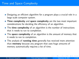
![Space Complexity
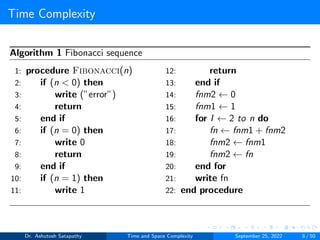
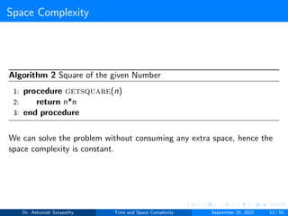
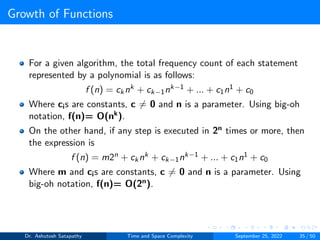
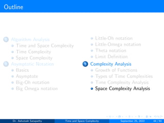
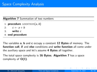
Algorithm 3 Sum of array elements
1: procedure calculate sum(A, n)
2: sum ← 0
3: for i ← 0 to n − 1 do
4: sum ← sum + A[i]
5: end for
6: end procedure
n, sum and i take constant sum of 3 units, but the variable A is an array,
it’s space consumption increases with the increase of input size n.
Dr. Ashutosh Satapathy Time and Space Complexity September 25, 2022 13 / 50](https://image.slidesharecdn.com/timeandspacecomplexity-220925154920-eed5cfac/85/Time-and-Space-Complexity-13-320.jpg)
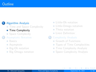
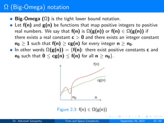
![O (Big-Oh) notation
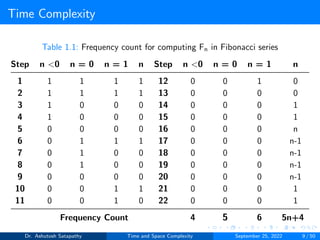
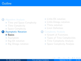
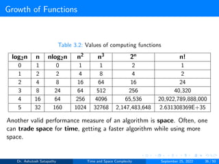
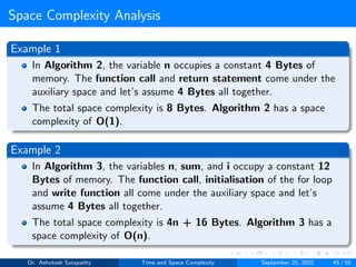
Question 1: Consider the function f(n) = 6n+ 135. Clearly. f(n) is
non-negative for all integers n ≥ 0. We wish to show that f(n)=O(n2).
According to the Big-oh definition, in order to show this we need to find
an integer n0, and a constant c > 0 such that for all integers, n ≥ n0, f(n)
= c(n2)
Answer: Suppose we choose c = 1, and f(n) = cn2.
⇒ 6n+135 = cn2 = n2 [Since c = 1] n2-6n-135 = 0
⇒ (n-15)(n+9) = 0
Since (n+9) > 0 for all values n ≥ 0, we conclude that (n-15) = 0
⇒ n0 = 15 for c = 1
For c = 2, n0 = (6 +
√
1116)/4 ≈ 9.9
For c = 4, n0 = (6 +
√
2196)/8 ≈ 6.7
Dr. Ashutosh Satapathy Time and Space Complexity September 25, 2022 20 / 50](https://image.slidesharecdn.com/timeandspacecomplexity-220925154920-eed5cfac/85/Time-and-Space-Complexity-20-320.jpg)
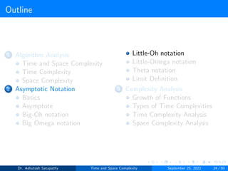
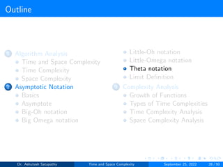
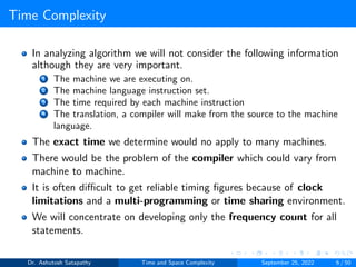
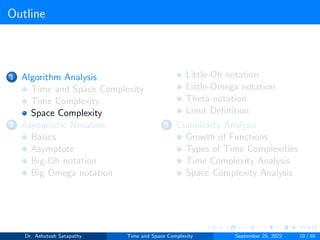
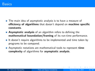
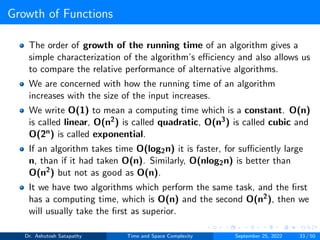
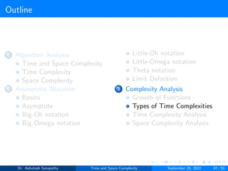
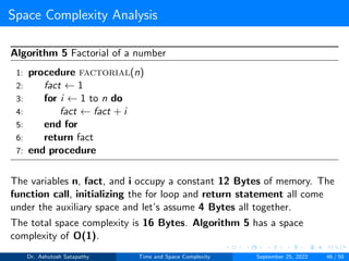
![Limit Definition
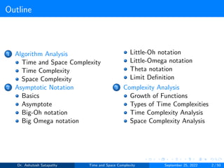
1 if f (n) ∈ O(g(n)) then limn→∞
f (n)
g(n) ∈ [0, ∞)
2 if f (n) ∈ o(g(n)) then limn→∞
f (n)
g(n) = 0
3 if f (n) ∈ Ω(g(n)) then limn→∞
f (n)
g(n) ∈ (0, ∞]
4 if f (n) ∈ ω(g(n)) then limn→∞
f (n)
g(n) = ∞
5 if f (n) ∈ θ(g(n)) then limn→∞
f (n)
g(n) ∈ (0, ∞)
Examples
1. n2 − 2n + 5 ∈ O(n3) ⇔ limn→∞
n2−2n+5
n3 = limn→∞
1
n − 2
n2 + 5
n3 = 0
2. n2 + 1 ∈ Ω(n) ⇔ limn→∞
n2+1
n = ∞
3. n2 + 3n + 4 ∈ θ(n2) ⇔ limn→∞
n2+3n+4
n2 = limn→∞(1 + 3
n + 4
n2 ) = 1
4. 7n + 8 ∈ o(n2) ⇔ limn→∞
7n+8
n2 = limn→∞(7
n + 8
n2 ) = 0
5. 4n + 6 ∈ ω(1) ⇔ limn→∞
4n+6
1 = ∞
Dr. Ashutosh Satapathy Time and Space Complexity September 25, 2022 31 / 50](https://image.slidesharecdn.com/timeandspacecomplexity-220925154920-eed5cfac/85/Time-and-Space-Complexity-31-320.jpg)
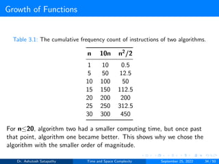
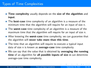
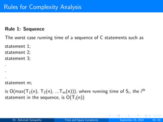
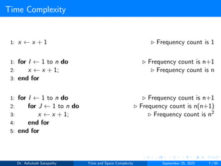
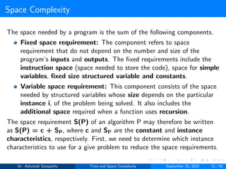
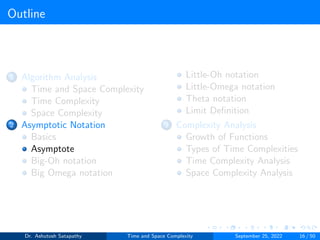
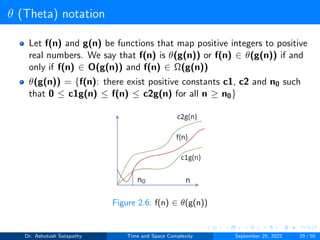
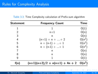
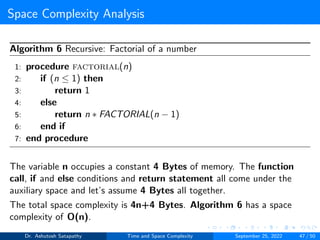
![Rules for Complexity Analysis
Algorithm 4 Prefix-sum
1: procedure prefix-sum(A, n)
2: for i ← n − 1 to 0 do
3: sum ← 0
4: for j ← 0 to i do
5: sum ← sum + A[j]
6: end for
7: A[i] ← sum
8: end for
9: end procedure
Dr. Ashutosh Satapathy Time and Space Complexity September 25, 2022 42 / 50](https://image.slidesharecdn.com/timeandspacecomplexity-220925154920-eed5cfac/85/Time-and-Space-Complexity-42-320.jpg)

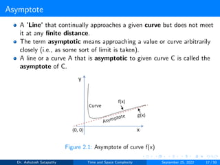
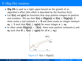
The document provides a comprehensive overview of time and space complexity in algorithm analysis, emphasizing their significance in determining algorithm efficiency. It explains various asymptotic notations such as big-oh, big-omega, and little-oh, including definitions and examples. Additionally, it covers the components of space complexity and offers analysis techniques for both time and space complexities.