Download to read offline

![29
Hash-JoinHash-Join
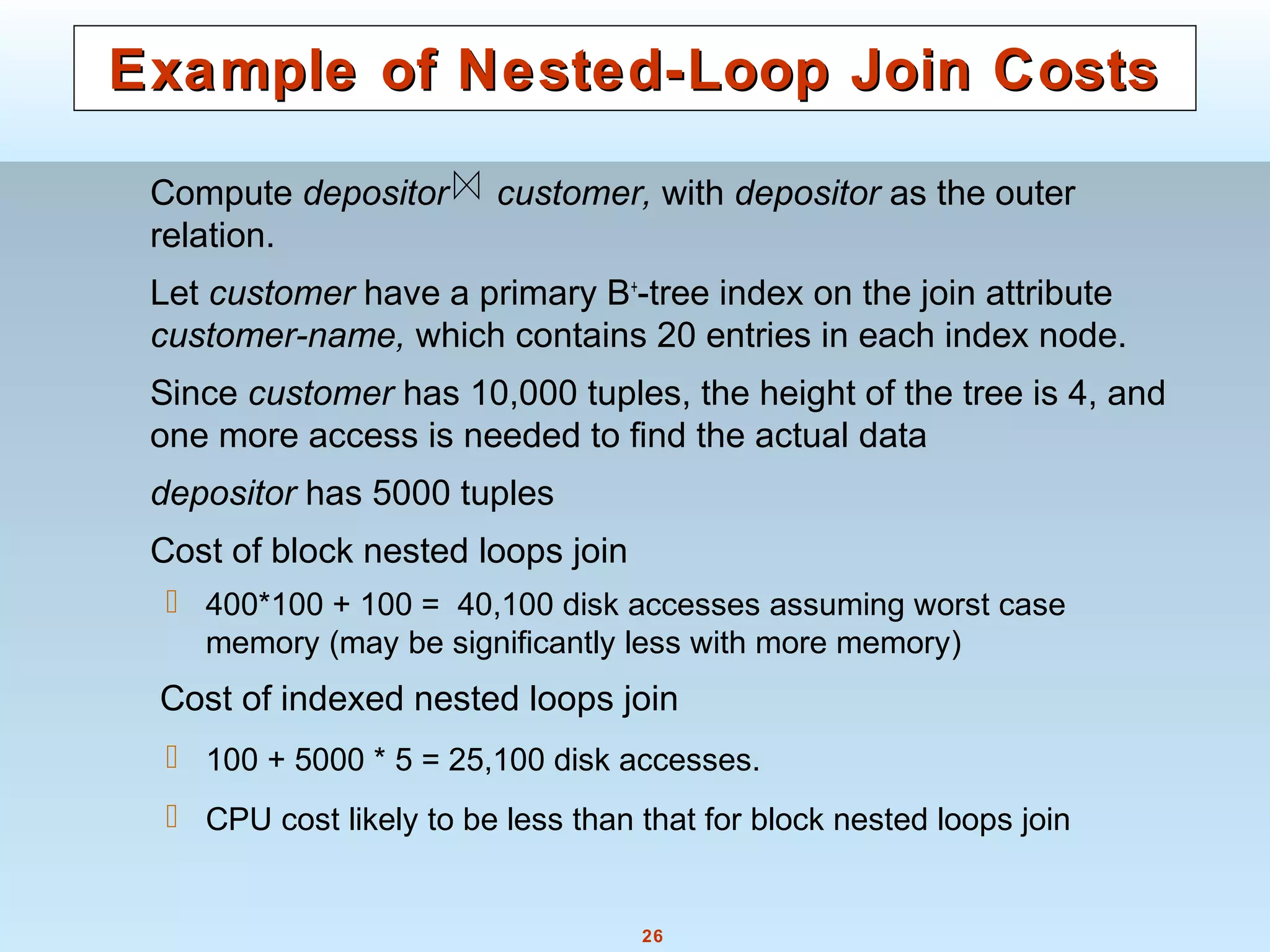
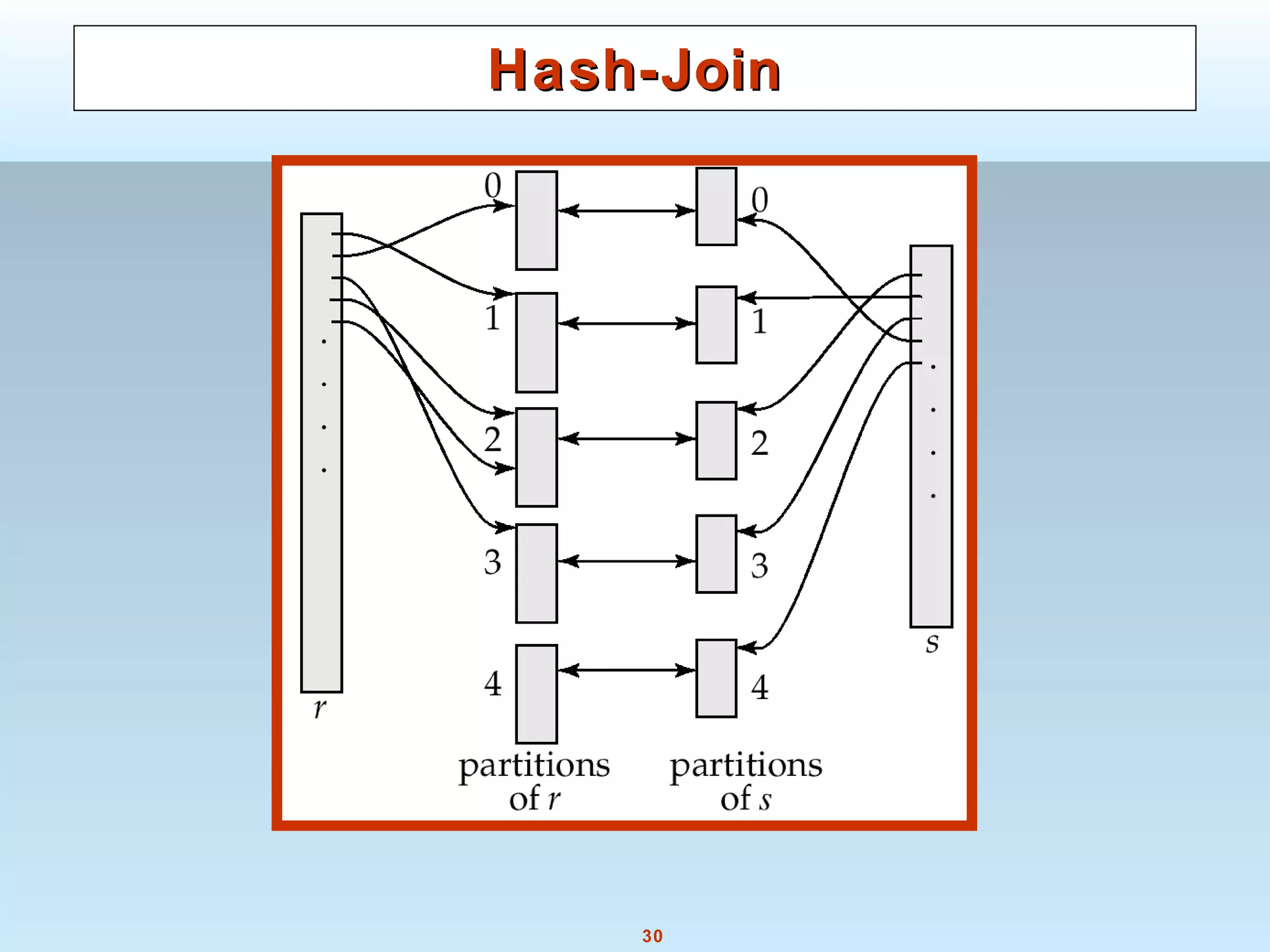
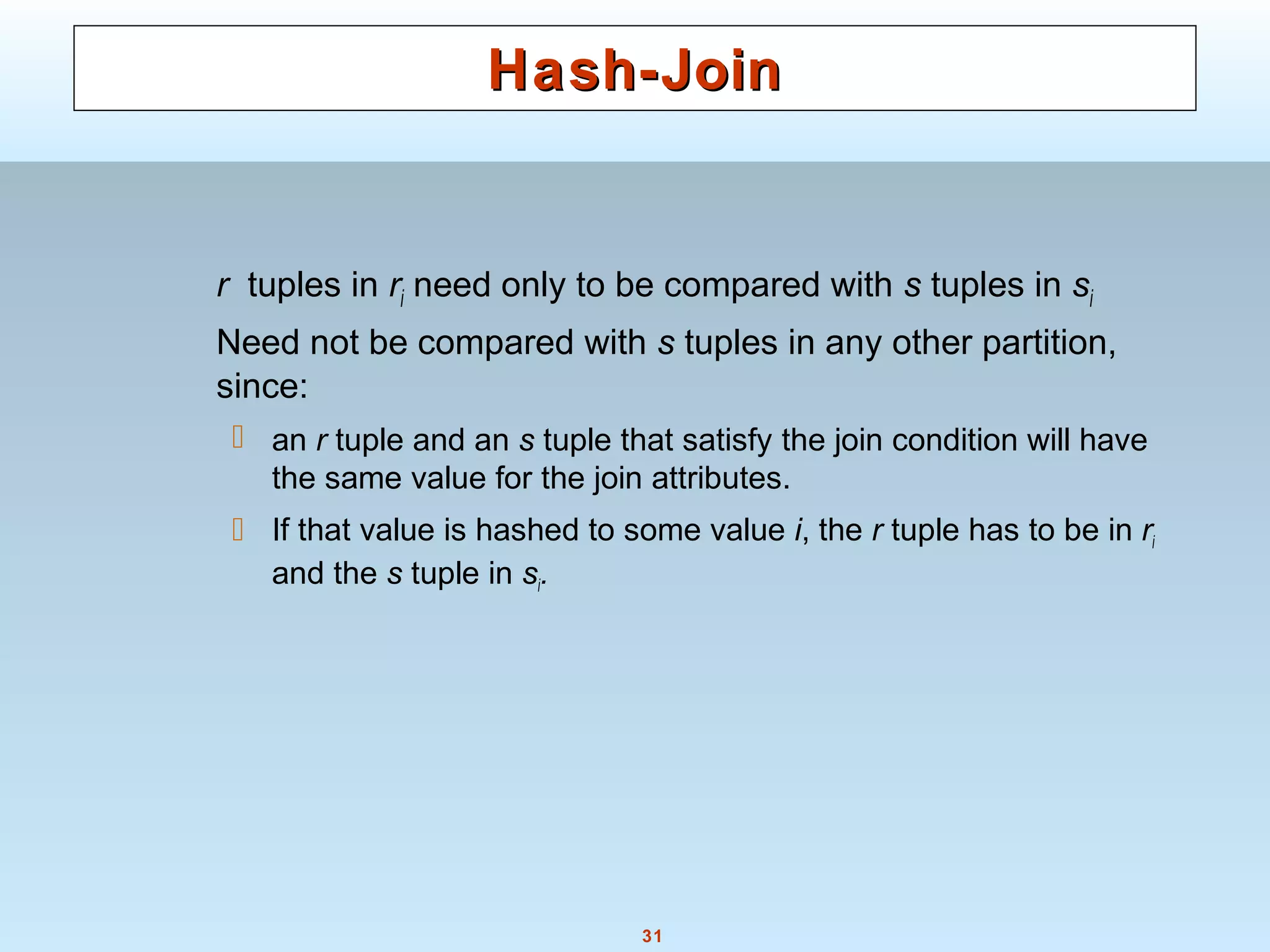
Applicable for equi-joins and natural joins.
A hash function h is used to partition tuples of both relations
h maps JoinAttrs values to {0, 1, ..., n}, where JoinAttrs denotes
the common attributes of r and s used in the natural join.
r0, r1, . . ., rn denote partitions of r tuples
Each tuple tr ∈ r is put in partition ri where i = h(tr[JoinAttrs]).
r0,, r1. . ., rn denotes partitions of s tuples
Each tuple ts ∈s is put in partition si, where i = h(ts[JoinAttrs]).
Note: In book, ri is denoted as Hri, si is denoted as Hsi and
nis denoted as nh.](https://image.slidesharecdn.com/28890lecture10-141217064709-conversion-gate02/75/28890-lecture10-29-2048.jpg)
![71
Join Order Optimization AlgorithmJoin Order Optimization Algorithm
procedure findbestplan(S)
if (bestplan[S].cost ≠ ∞)
return bestplan[S]
// else bestplan[S] has not been computed earlier, compute it now
for each non-empty subset S1 of S such that S1 ≠ S
P1= findbestplan(S1)
P2= findbestplan(S - S1)
A = best algorithm for joining results of P1 and P2
cost = P1.cost + P2.cost + cost of A
if cost < bestplan[S].cost
bestplan[S].cost = cost
bestplan[S].plan = “execute P1.plan; execute P2.plan;
join results of P1 and P2 using A”
return bestplan[S]](https://image.slidesharecdn.com/28890lecture10-141217064709-conversion-gate02/75/28890-lecture10-71-2048.jpg)
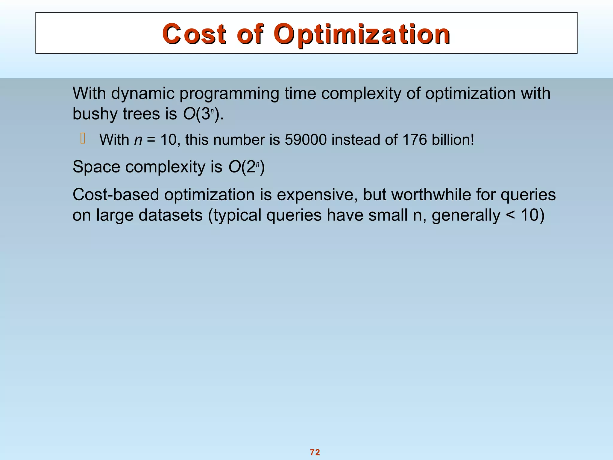
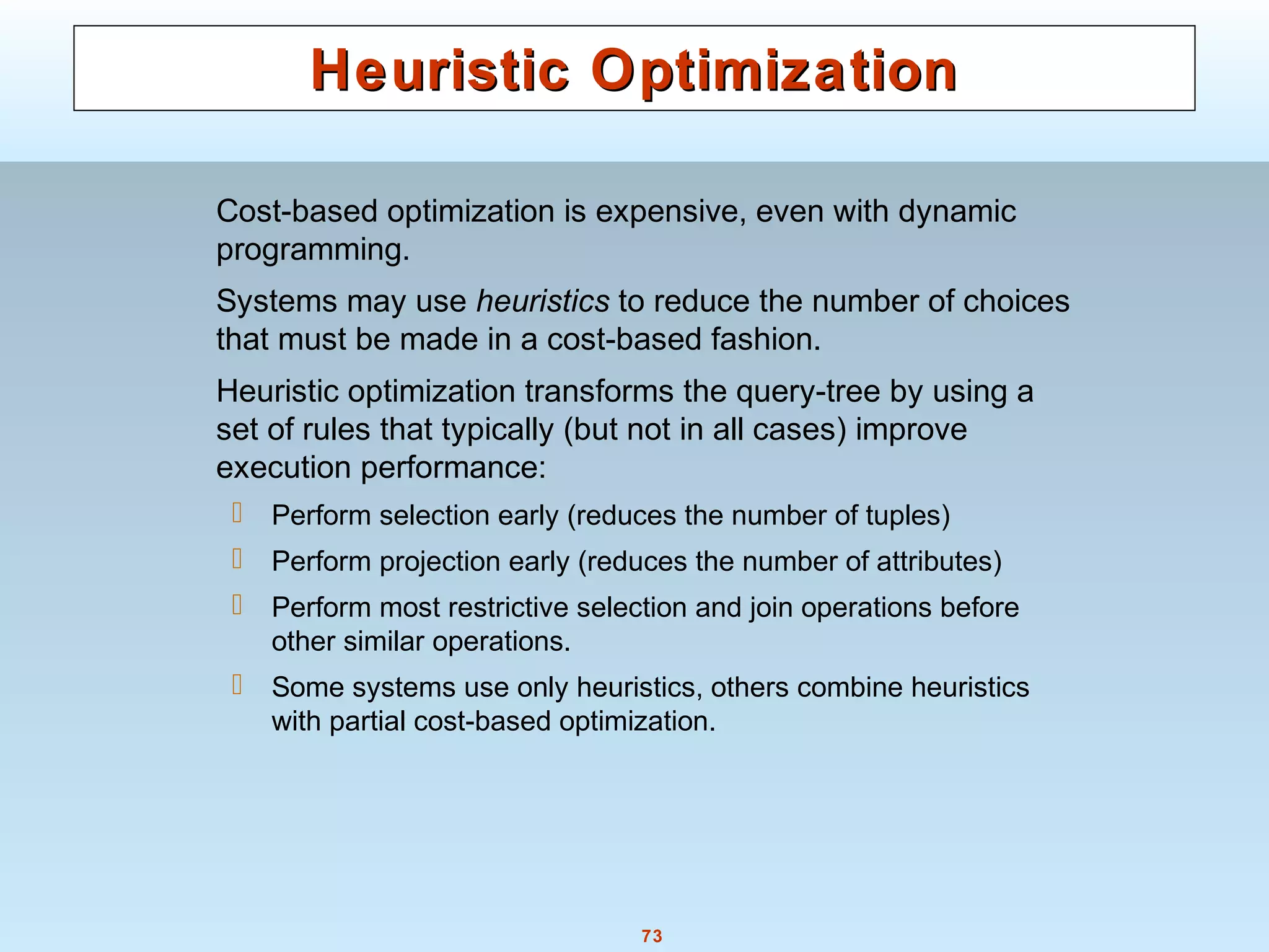
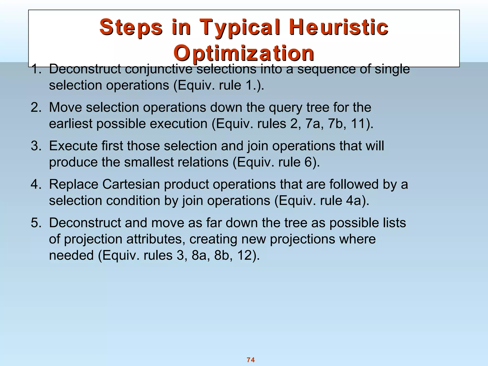

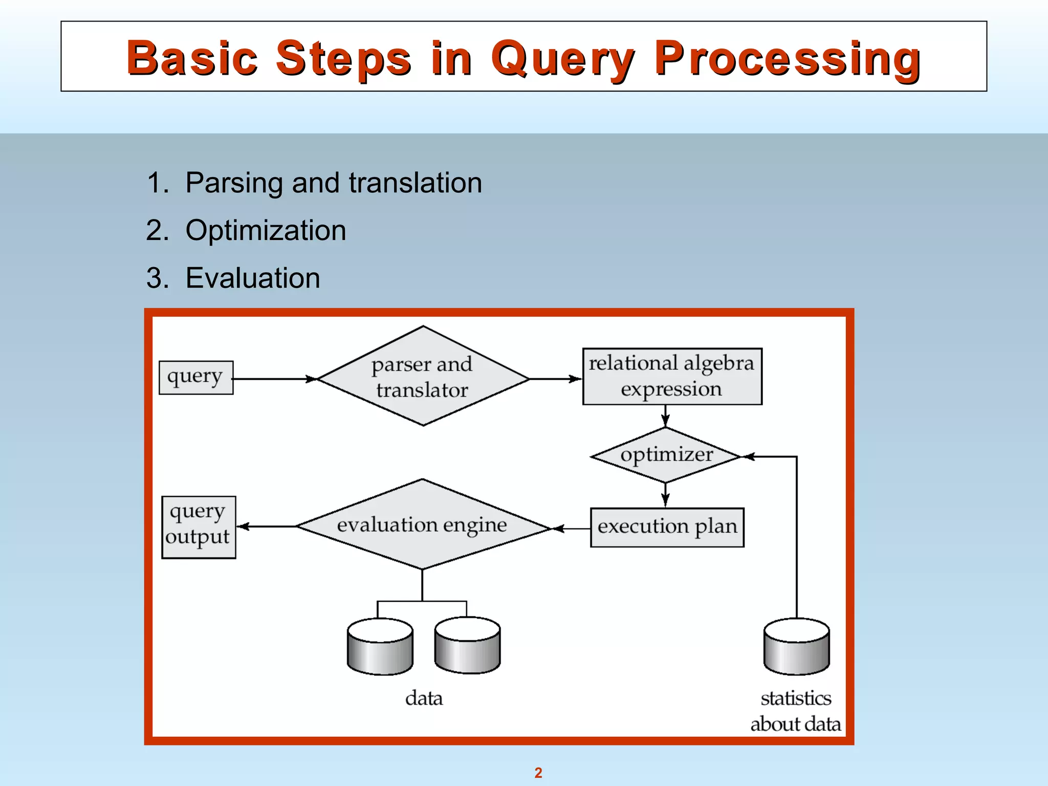
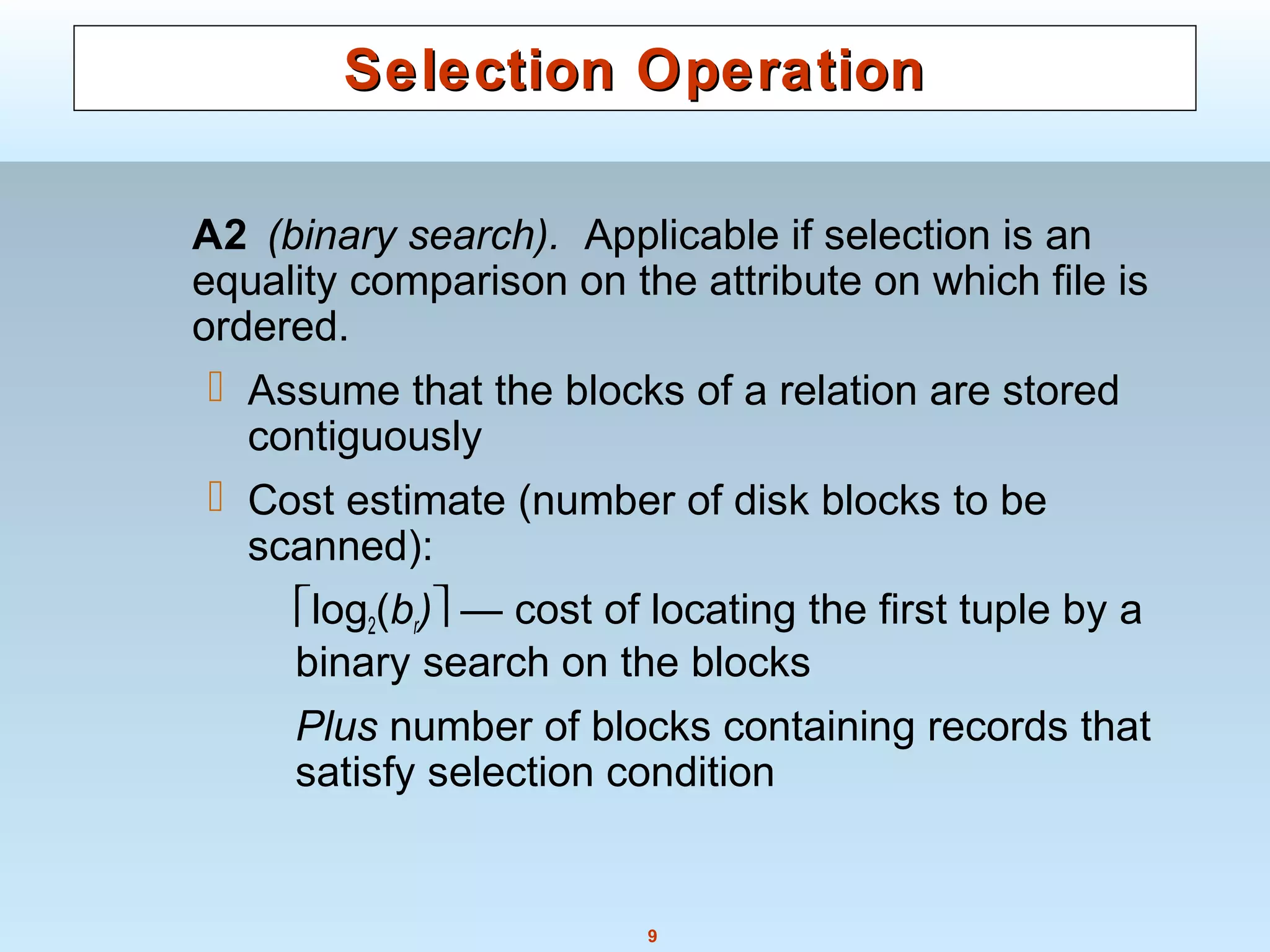
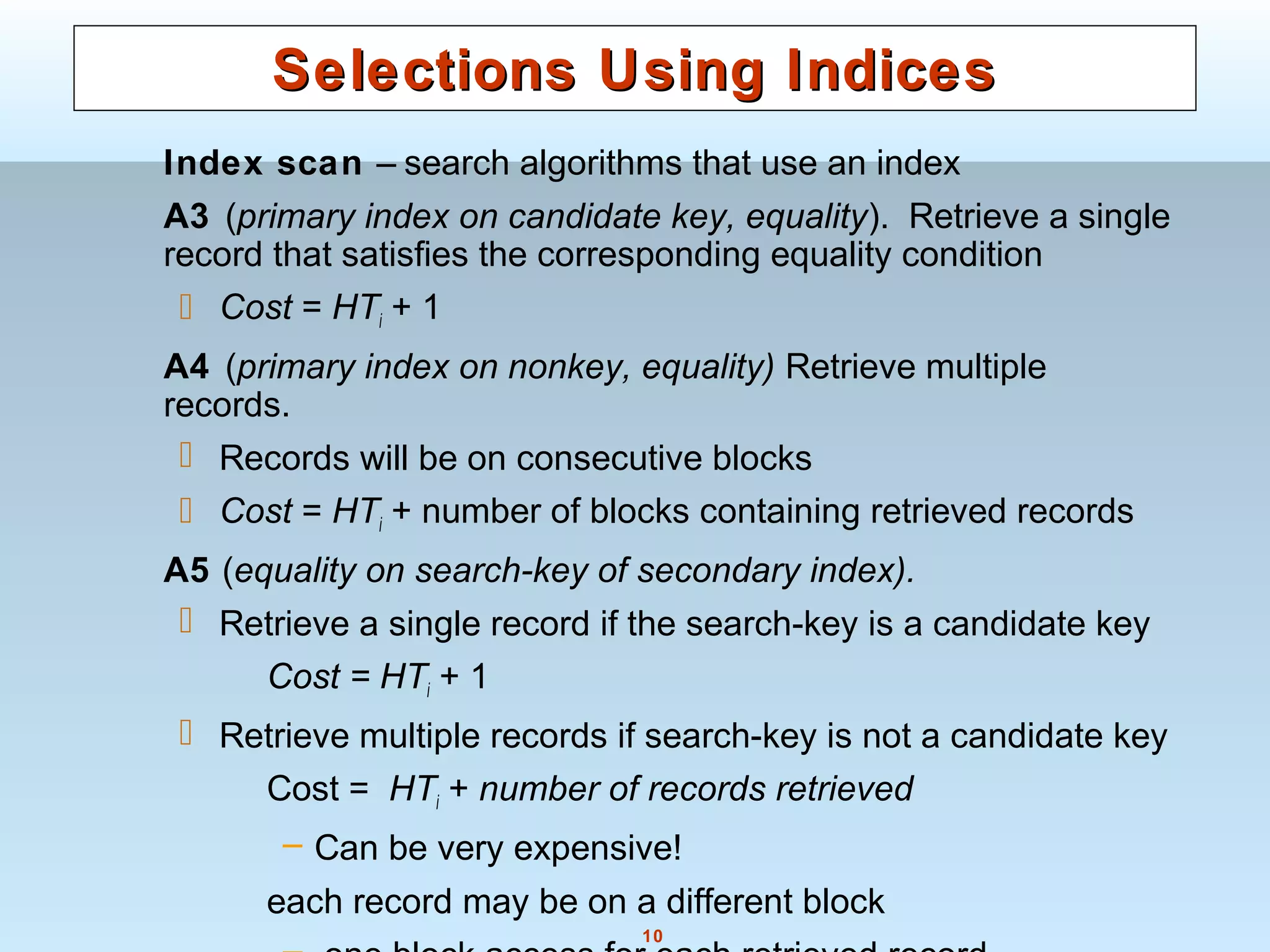
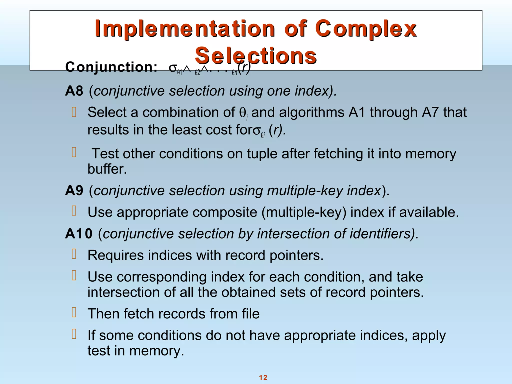
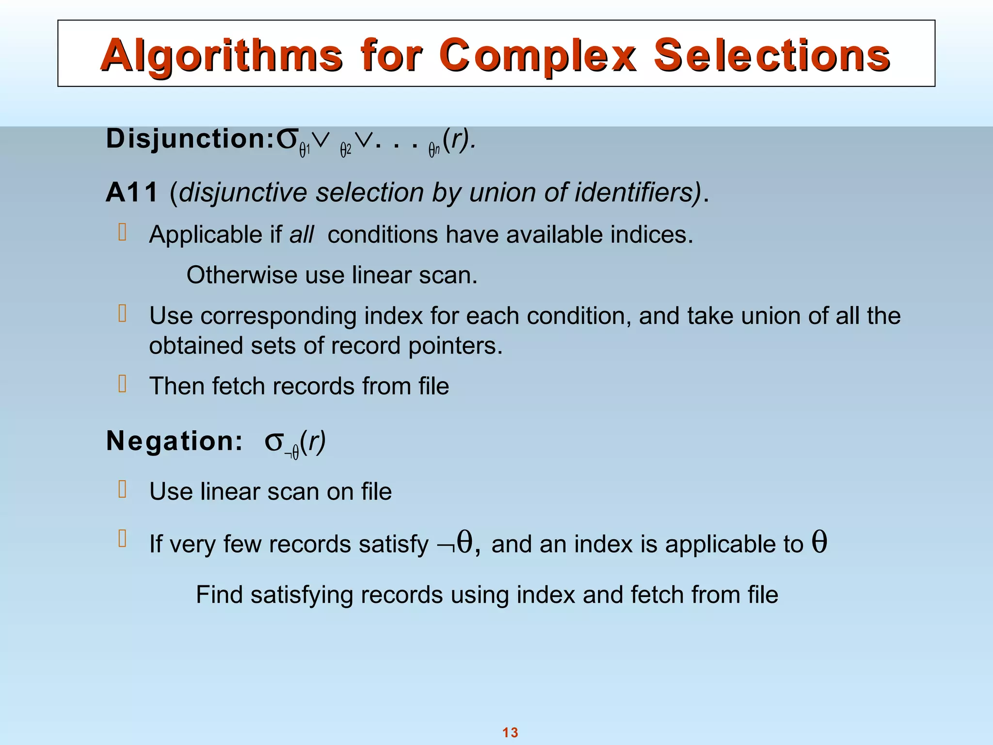
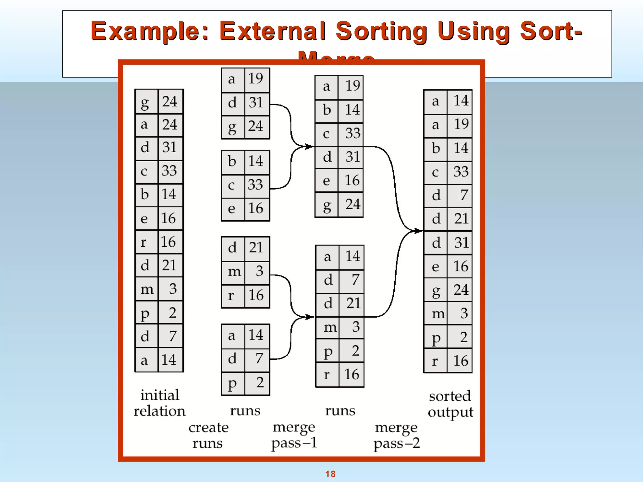
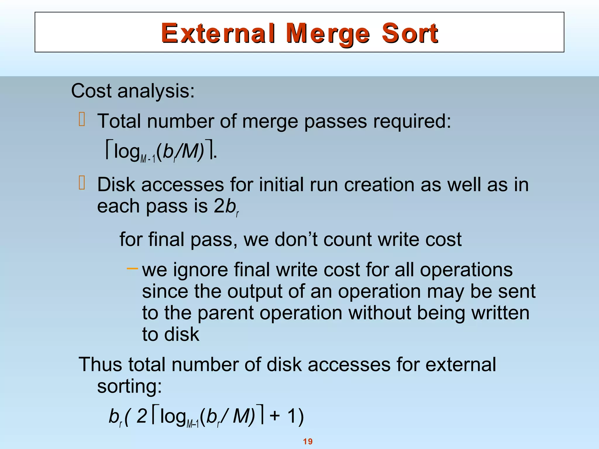
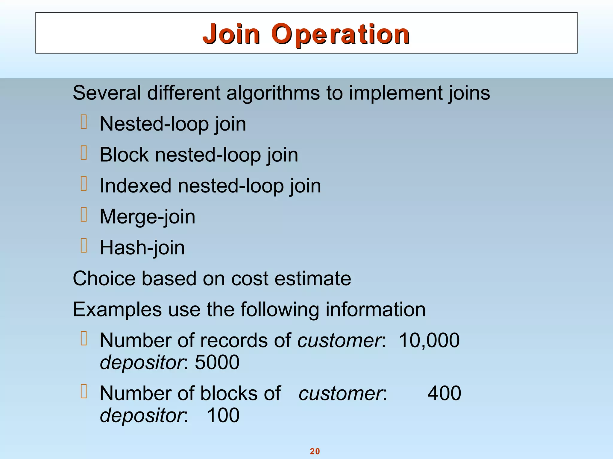
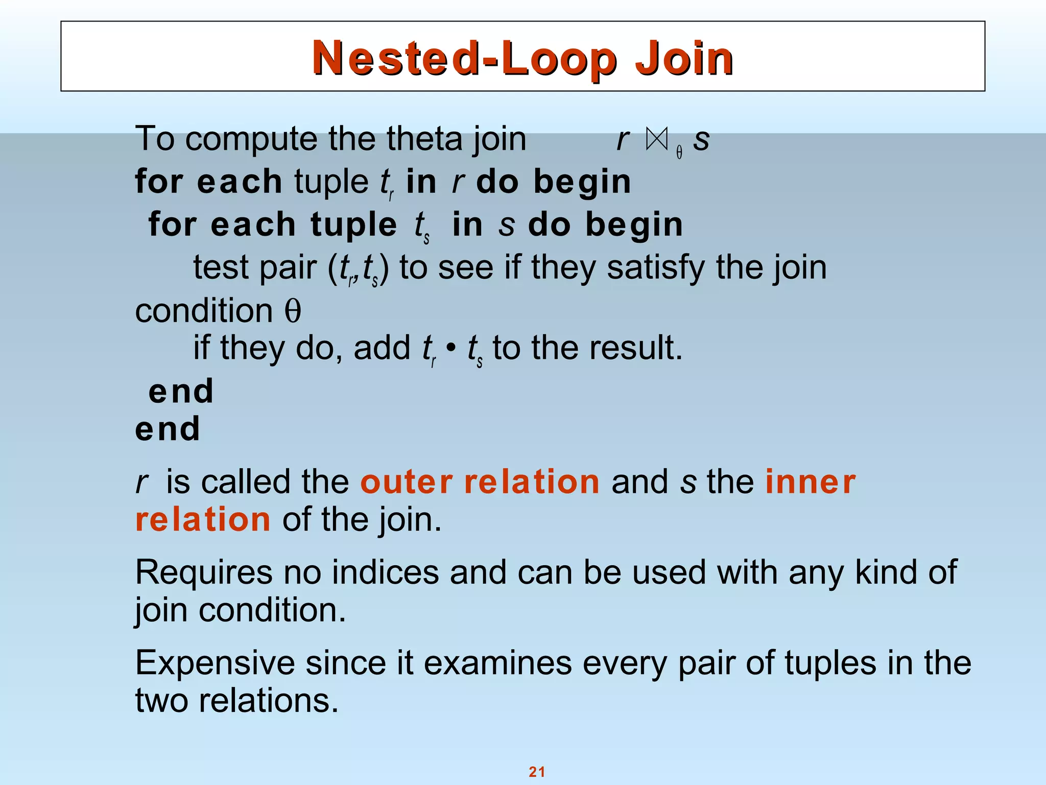
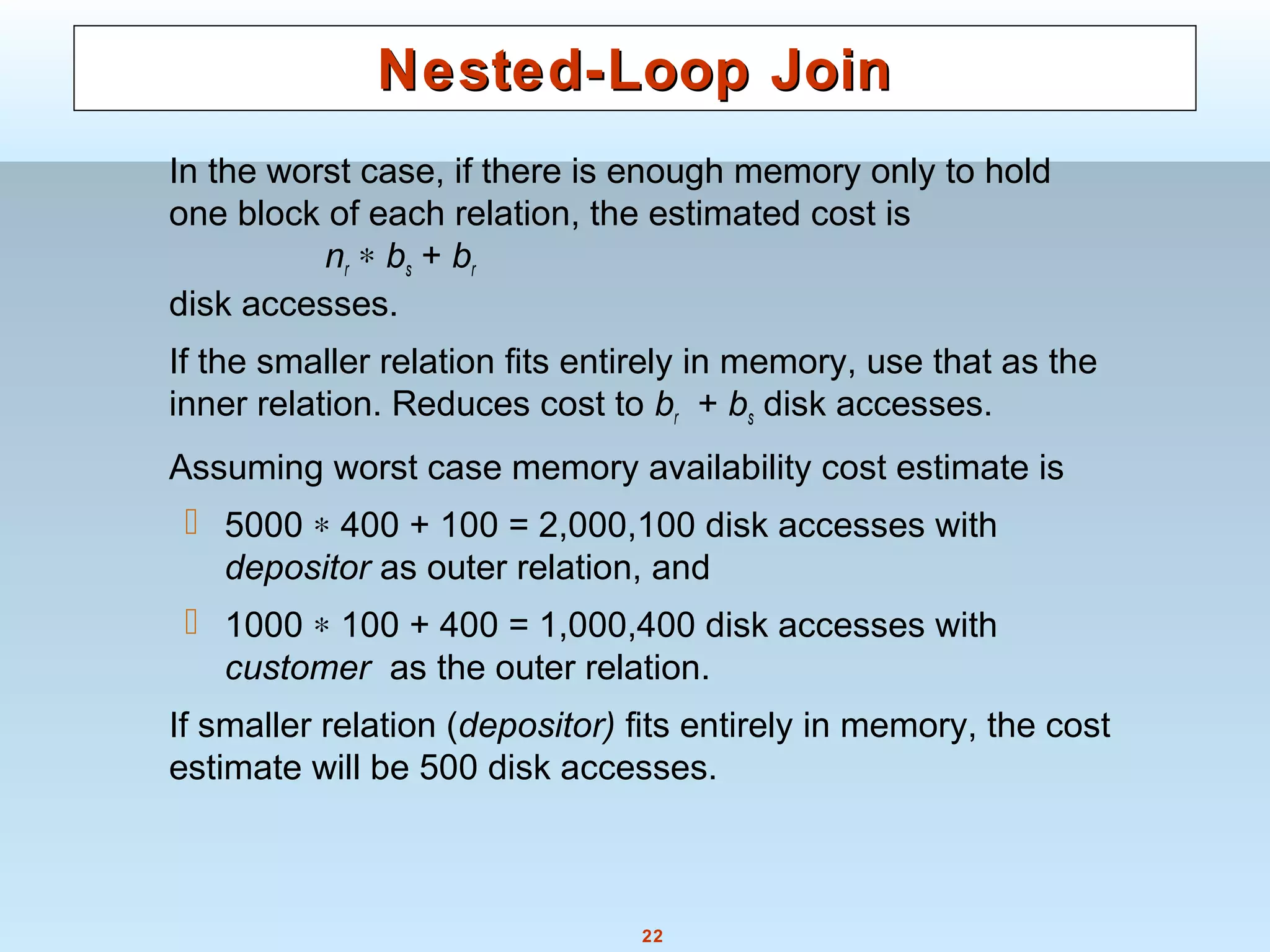
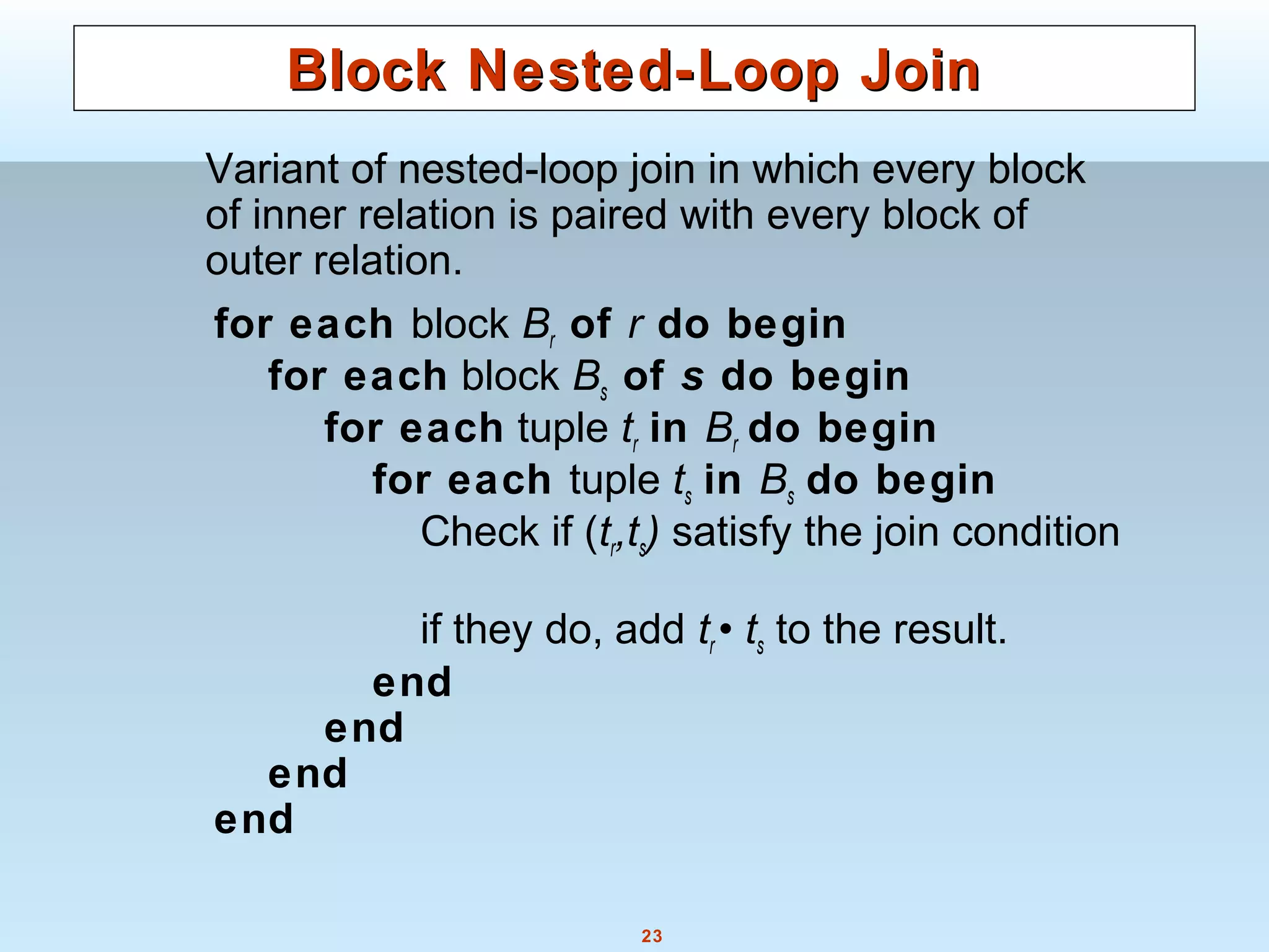
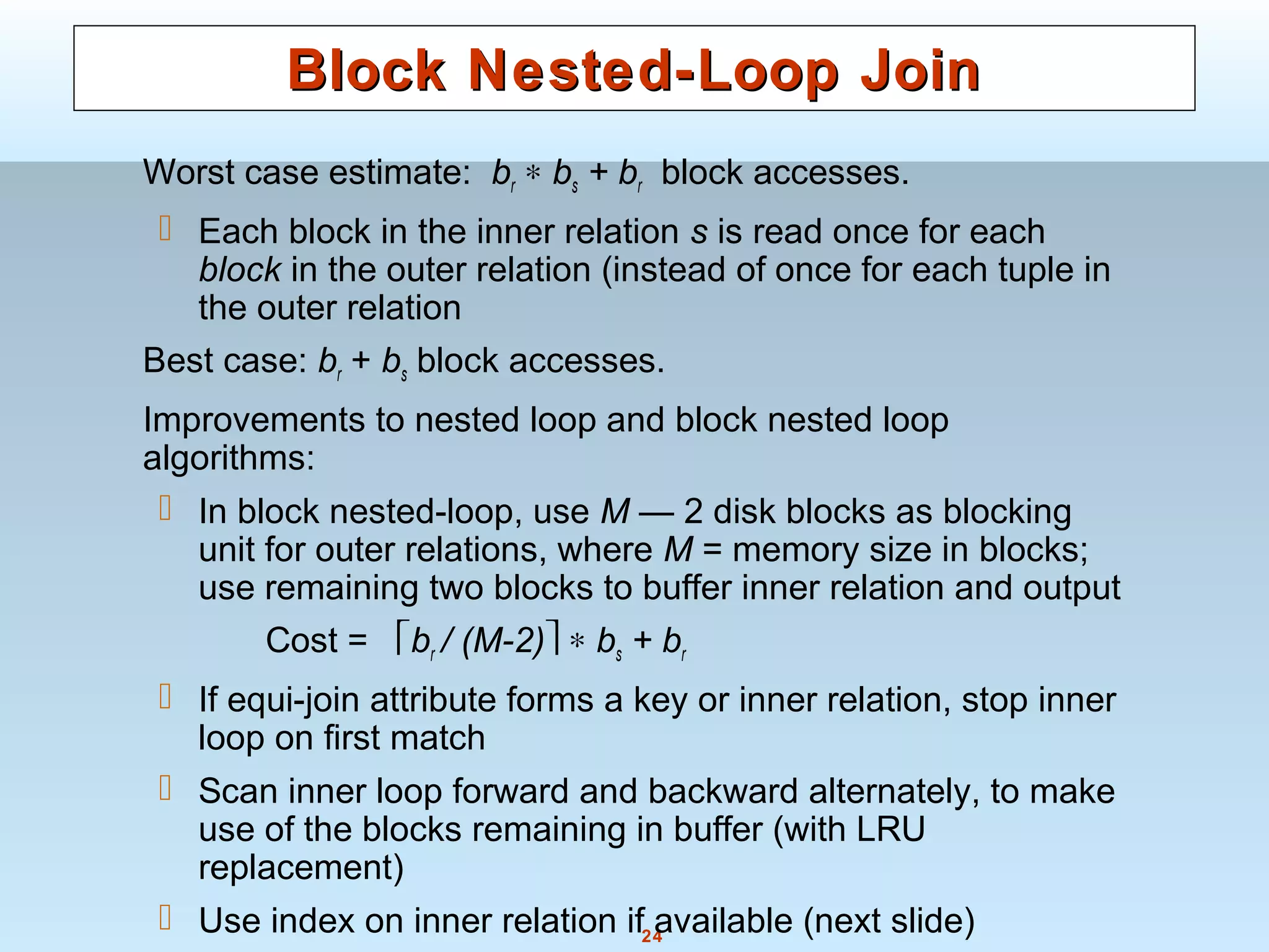
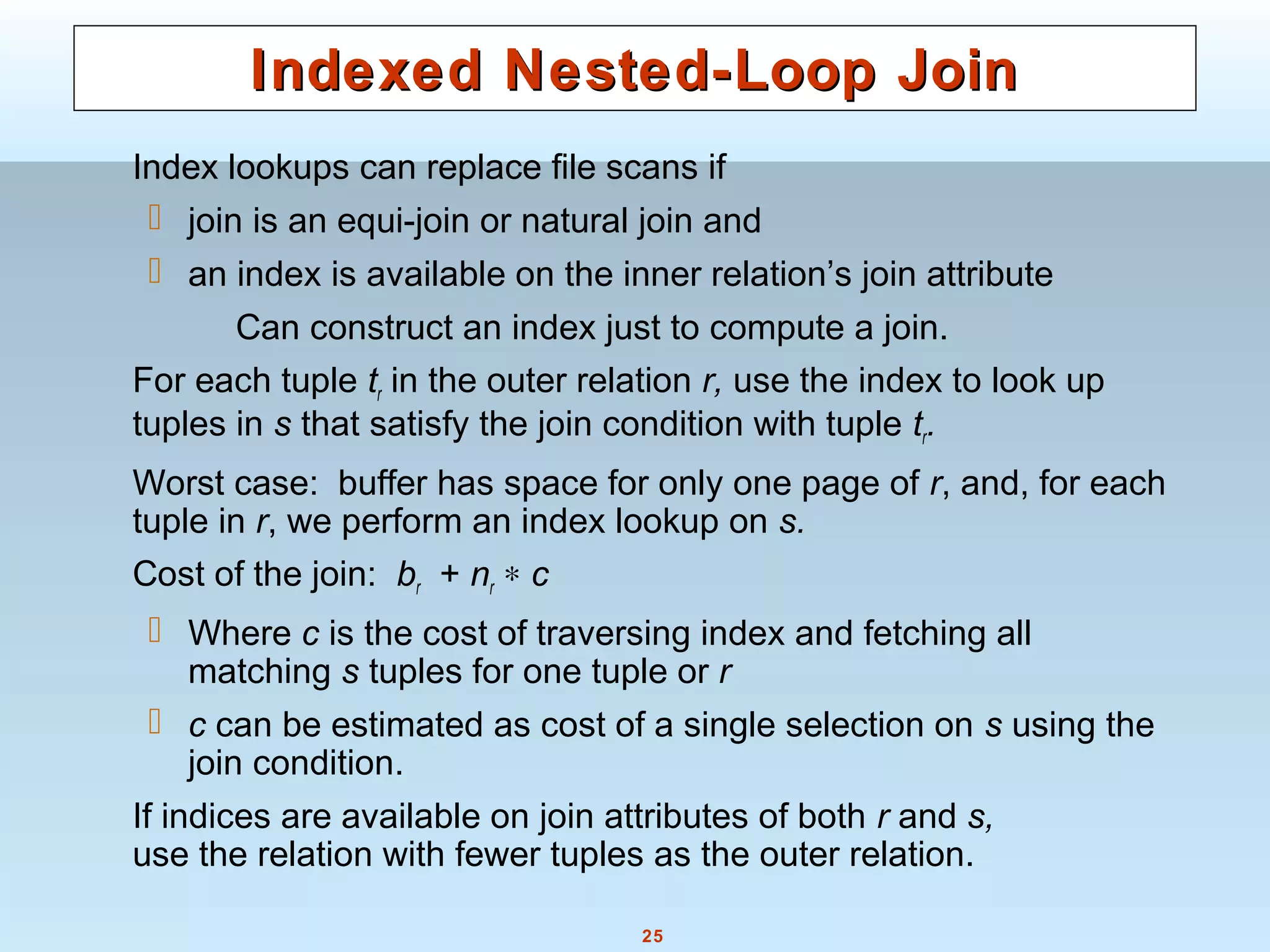
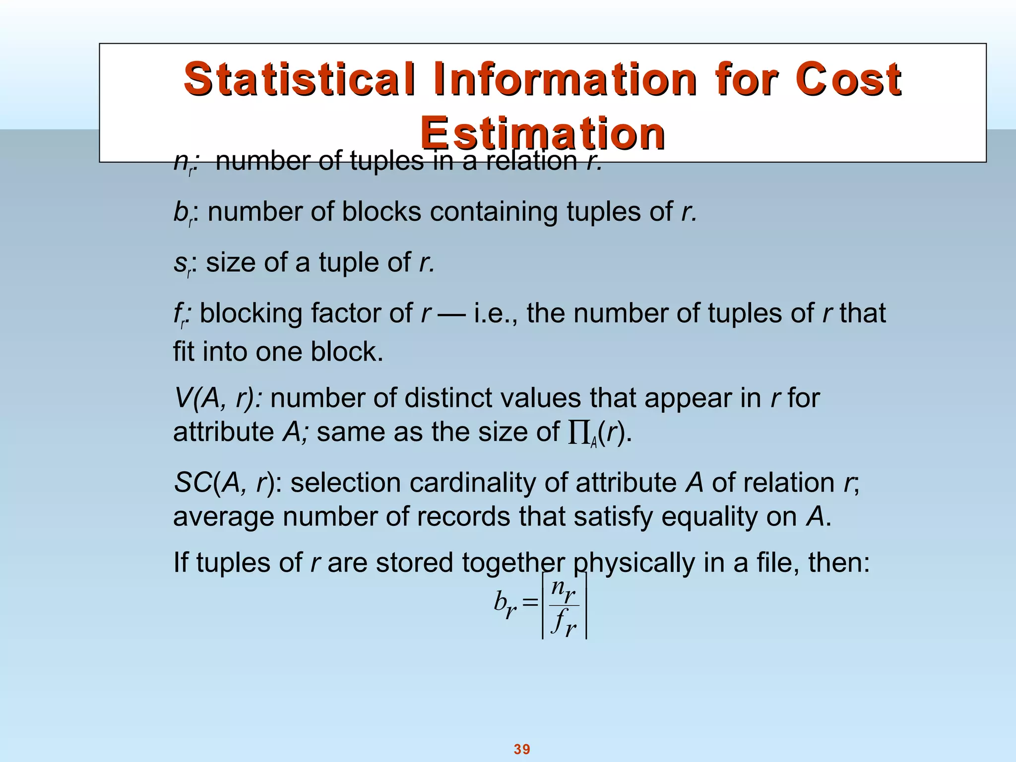
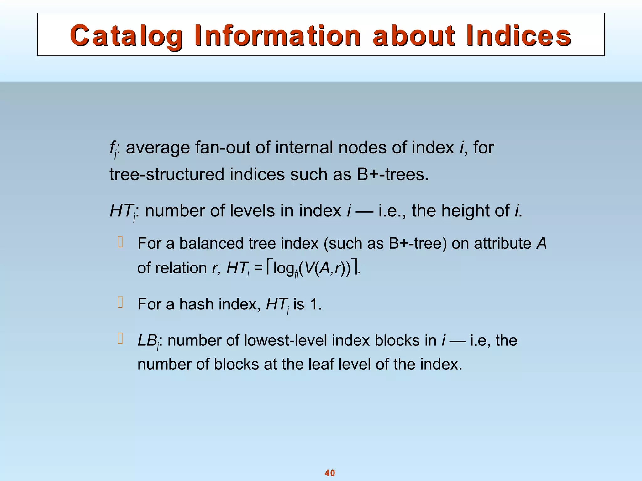
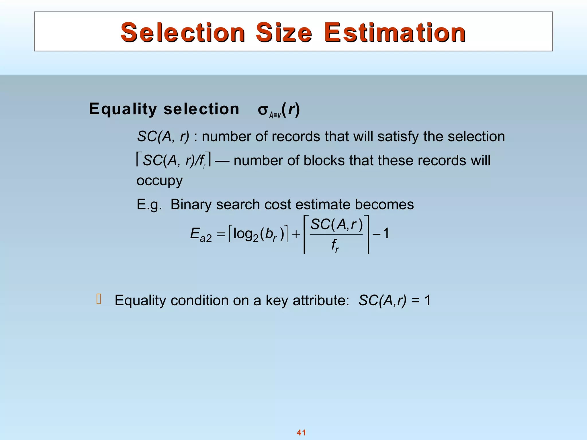
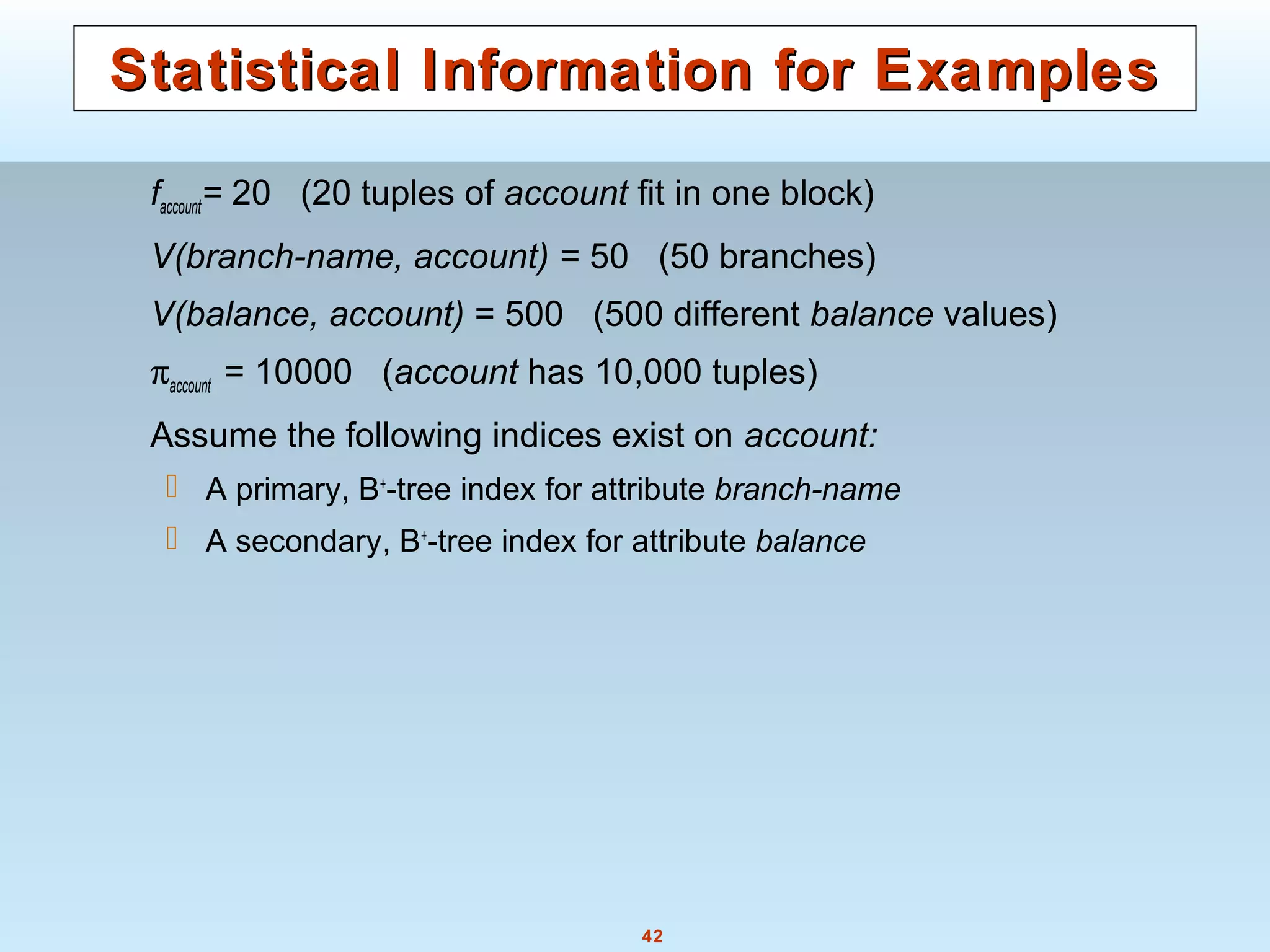
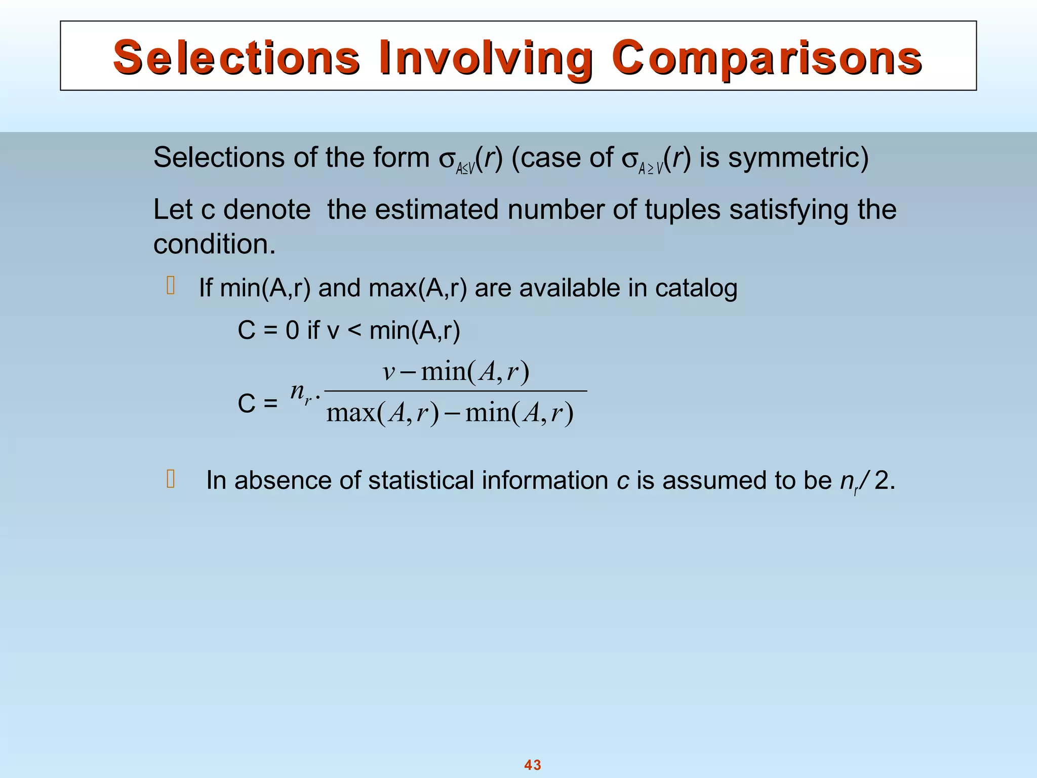
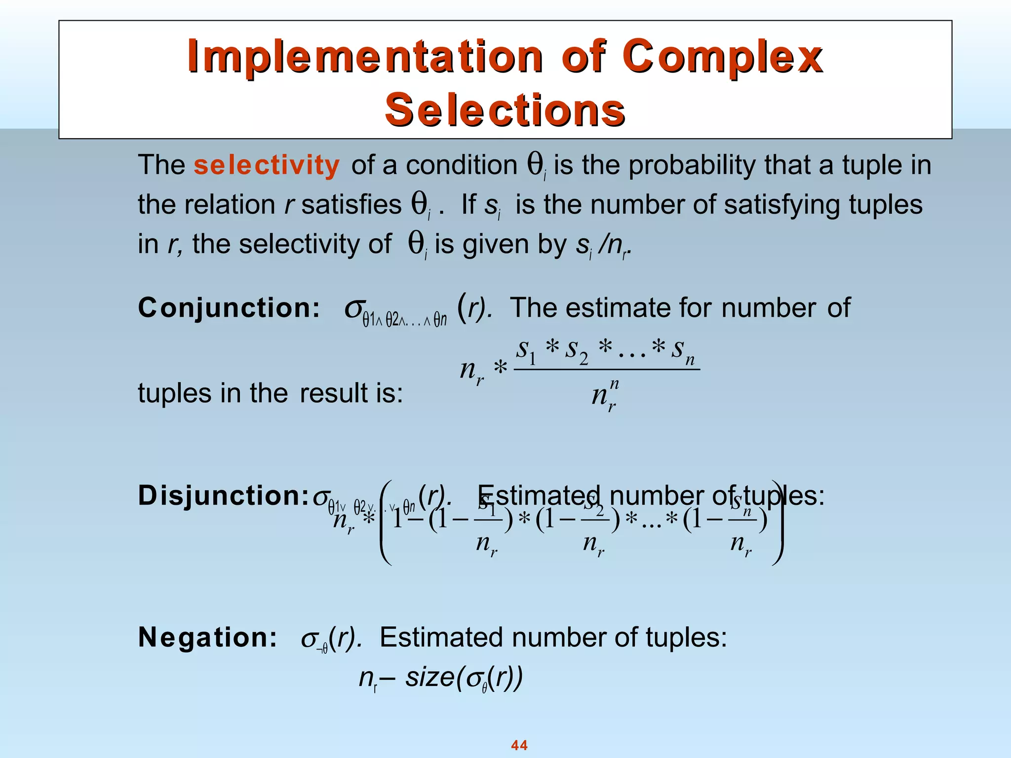
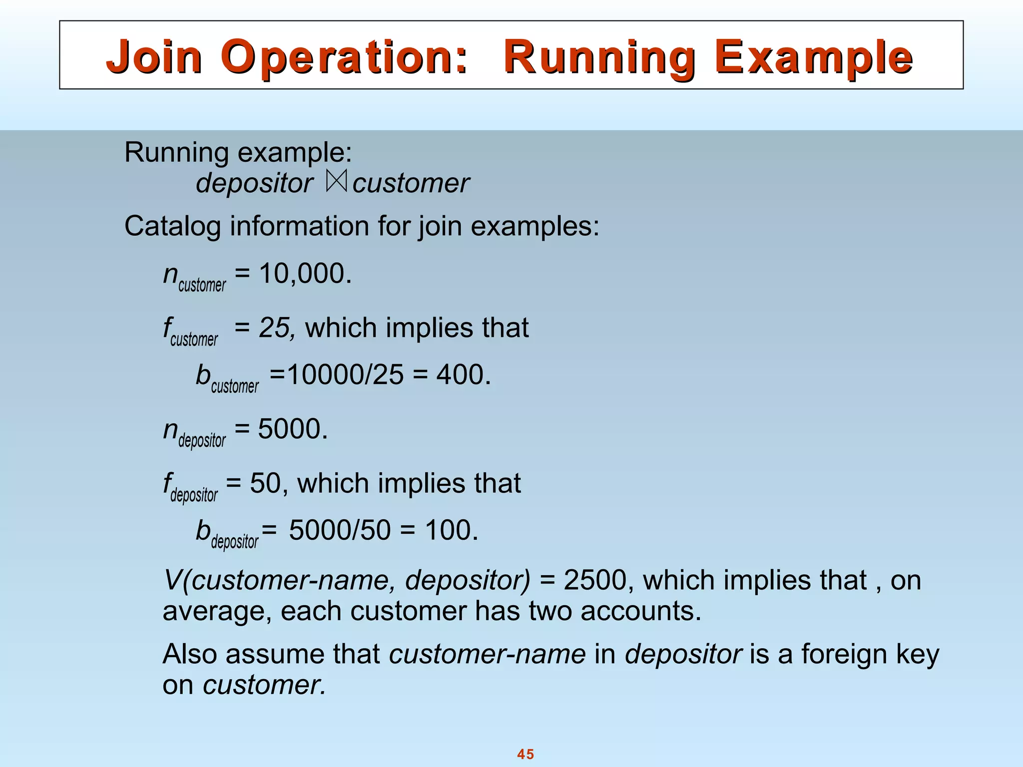
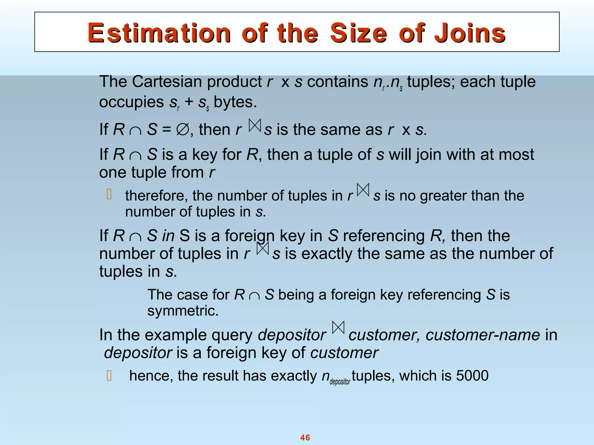
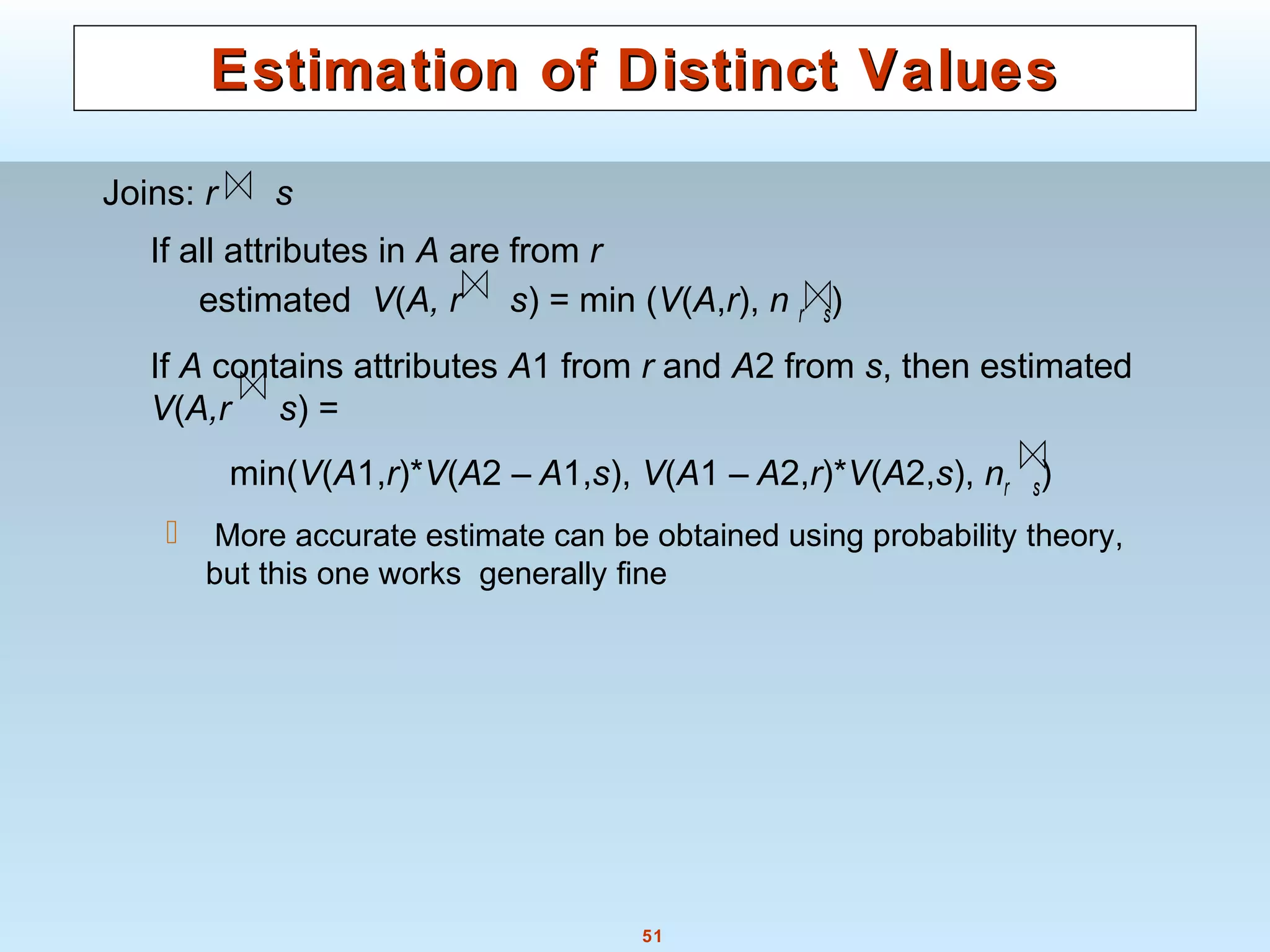
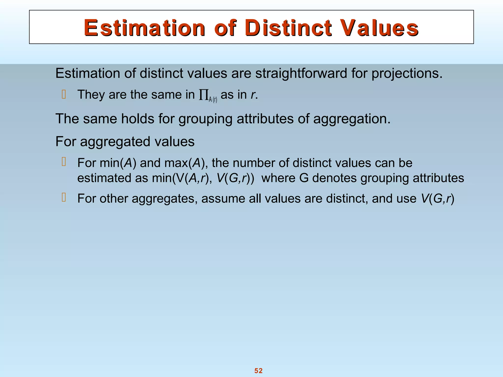
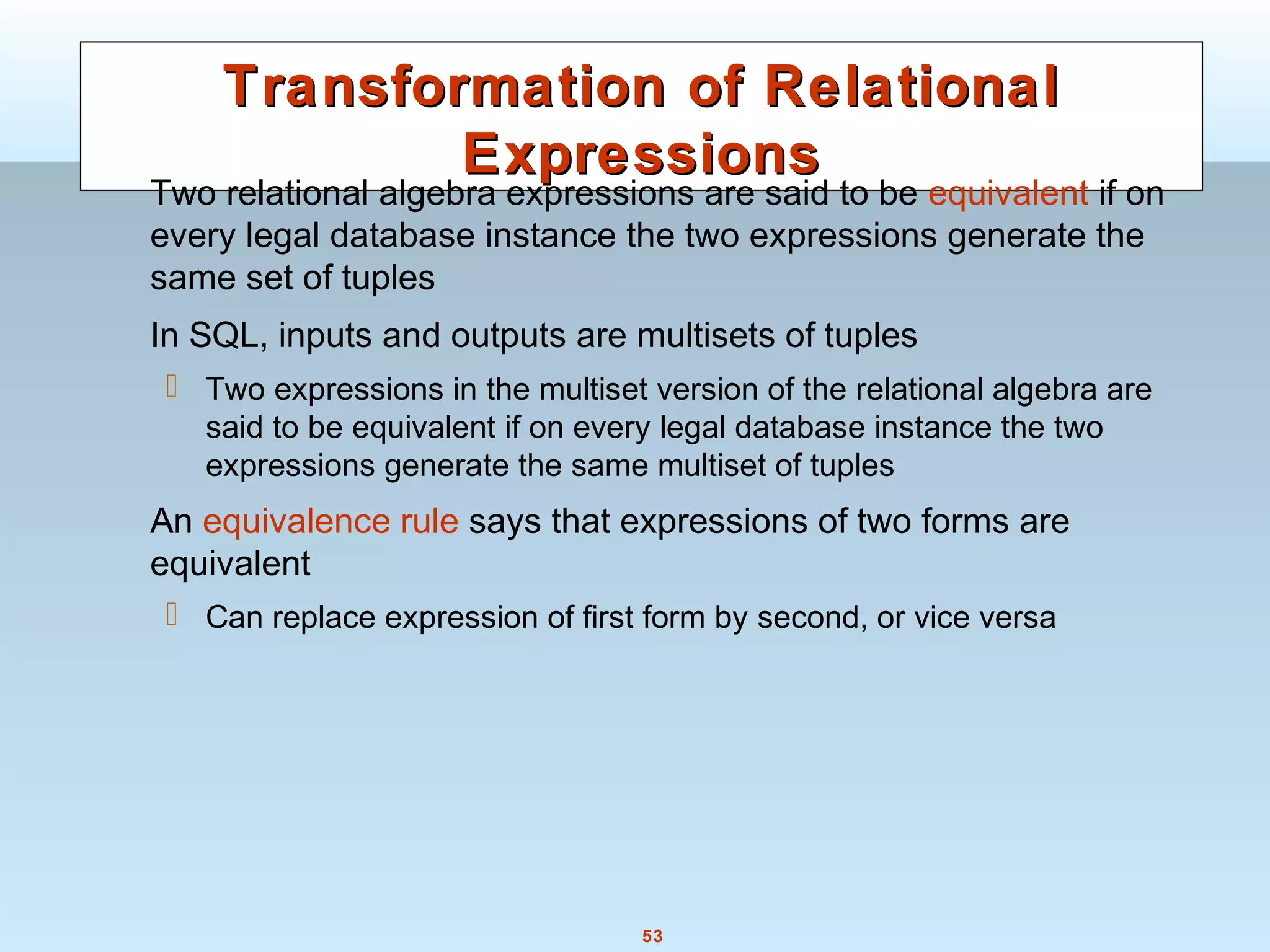
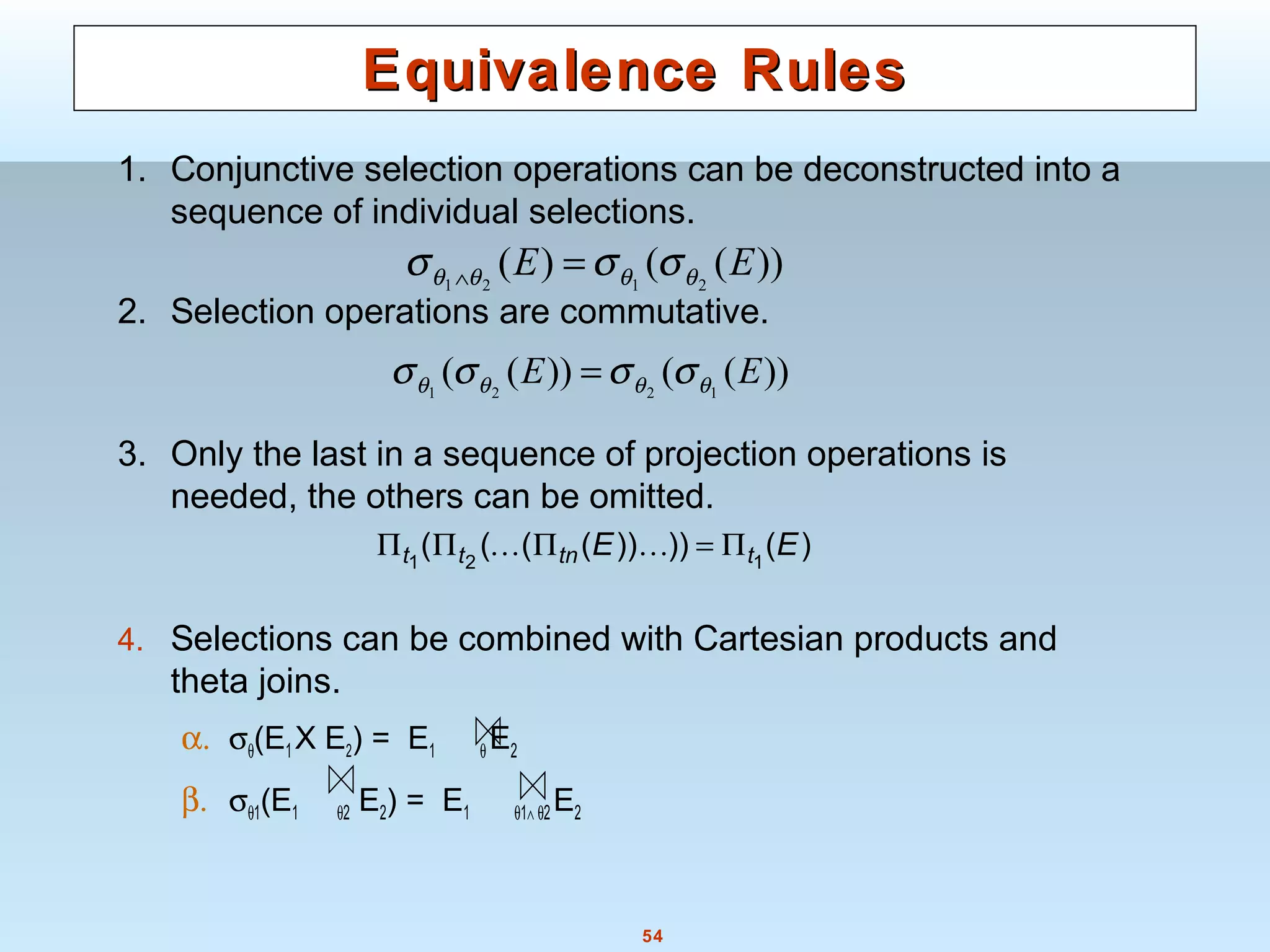
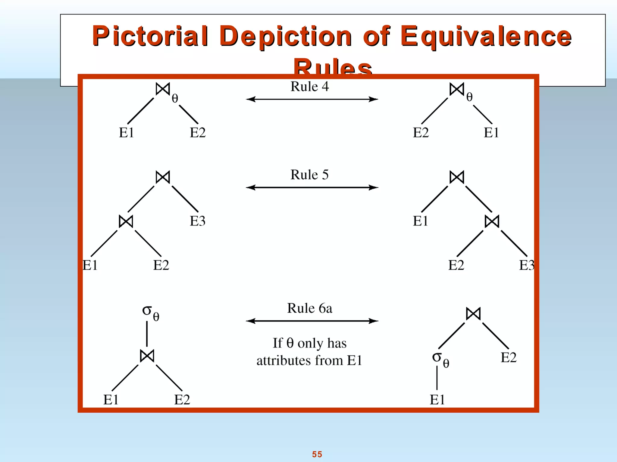
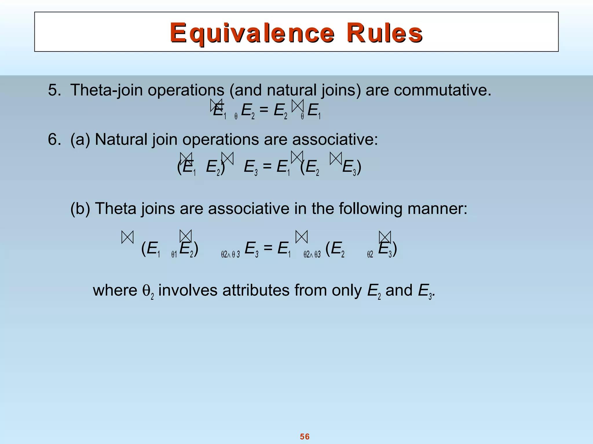
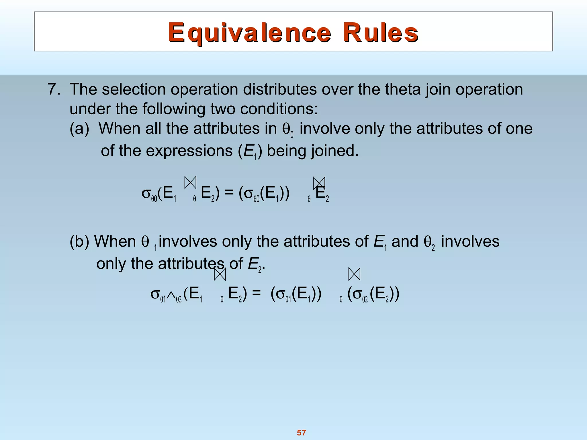
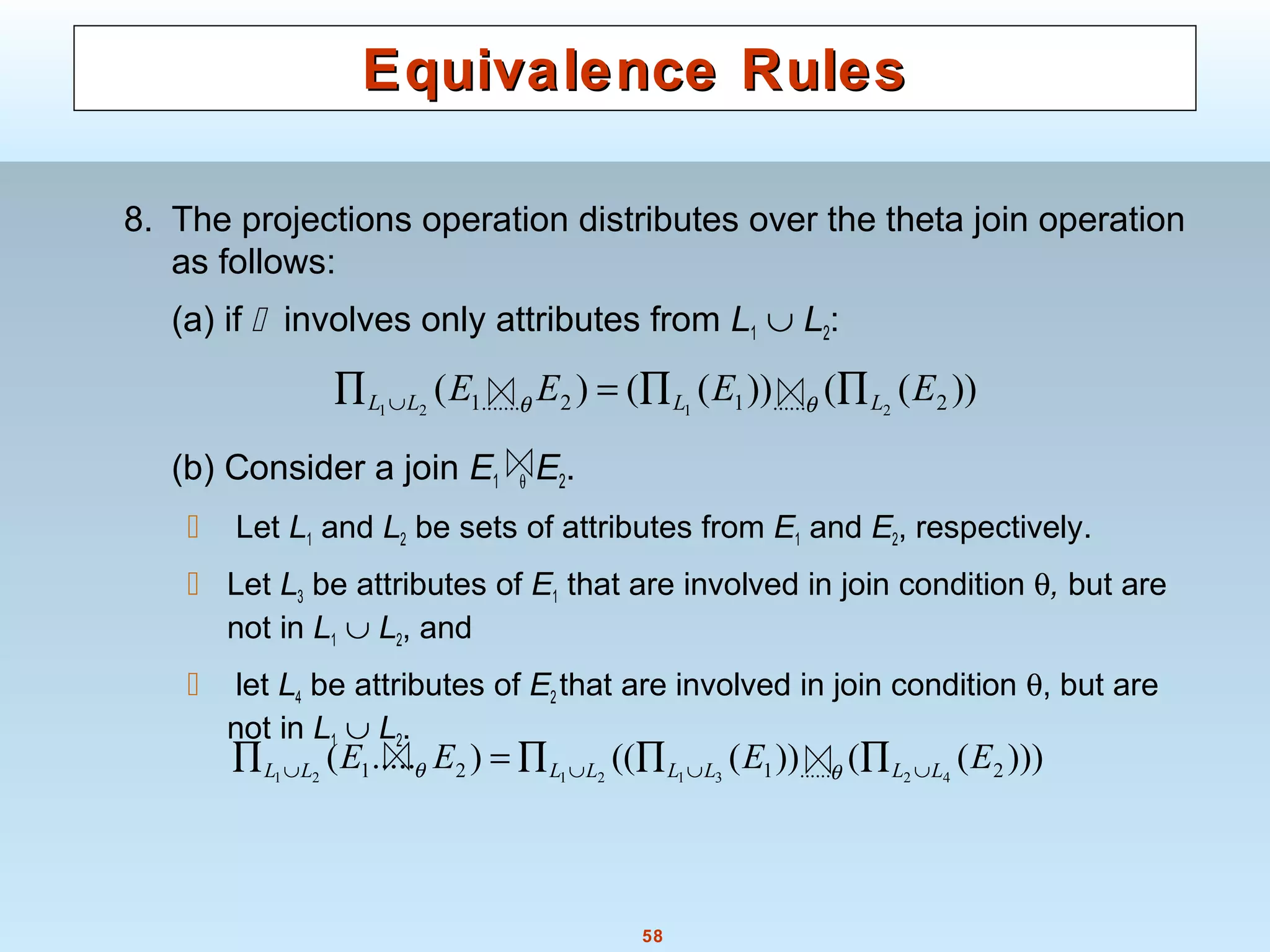
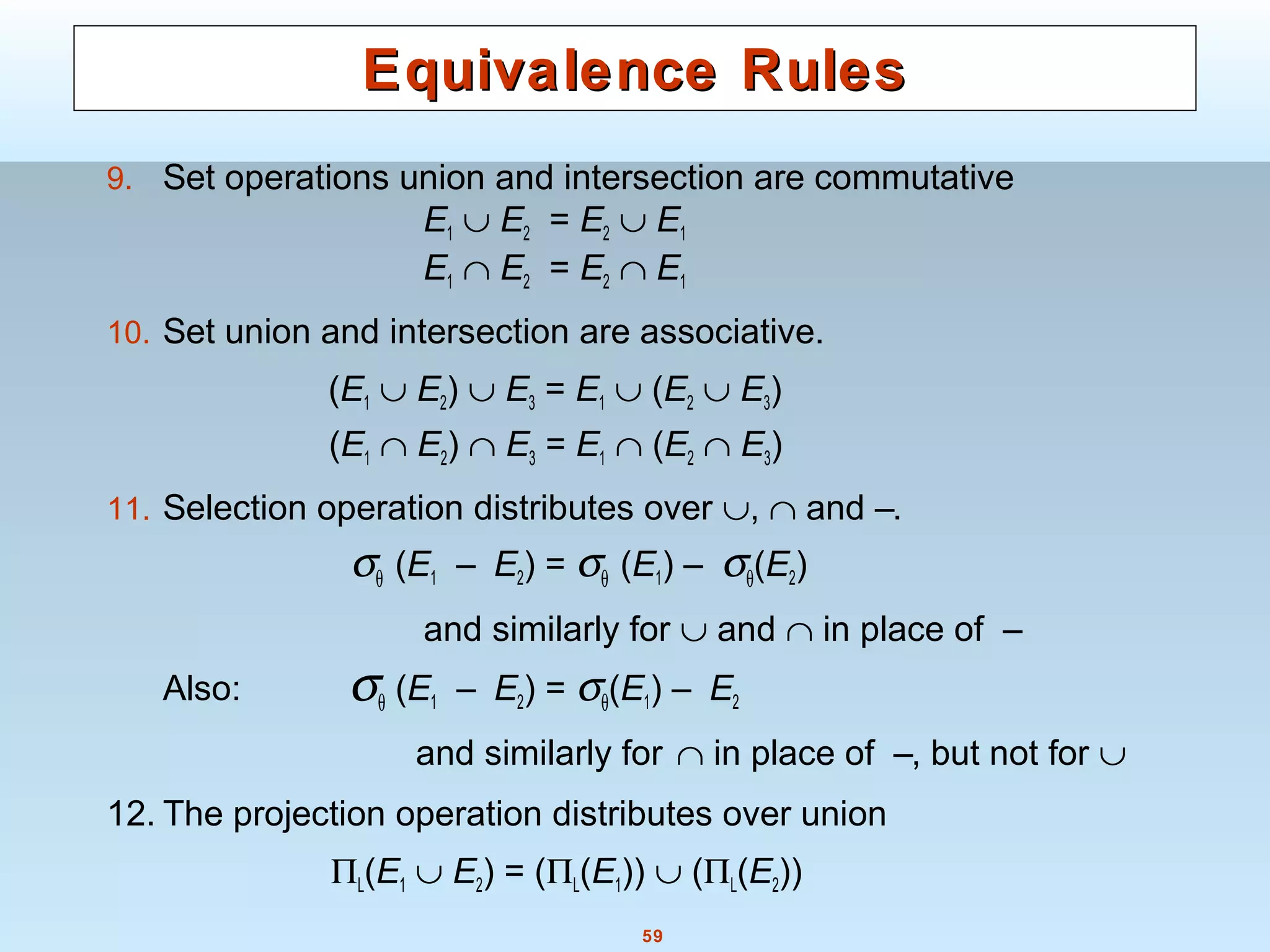
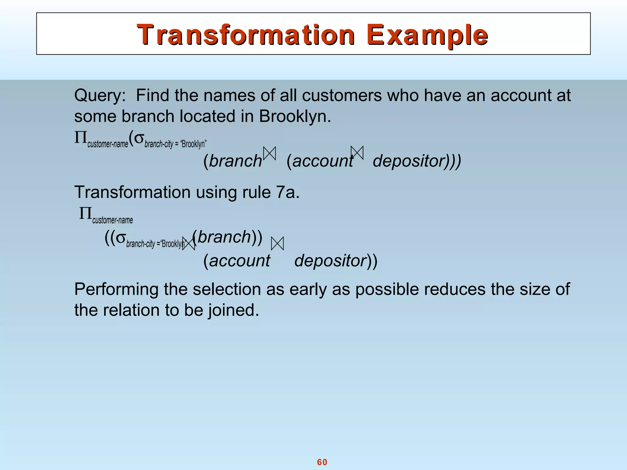
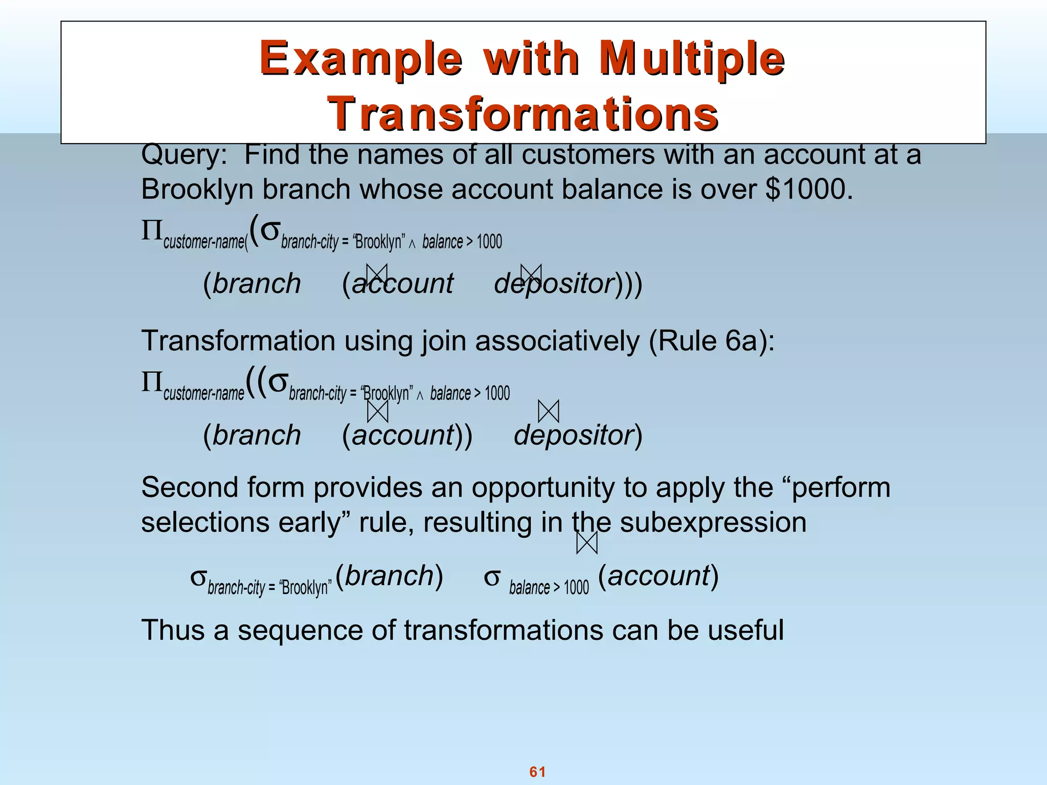
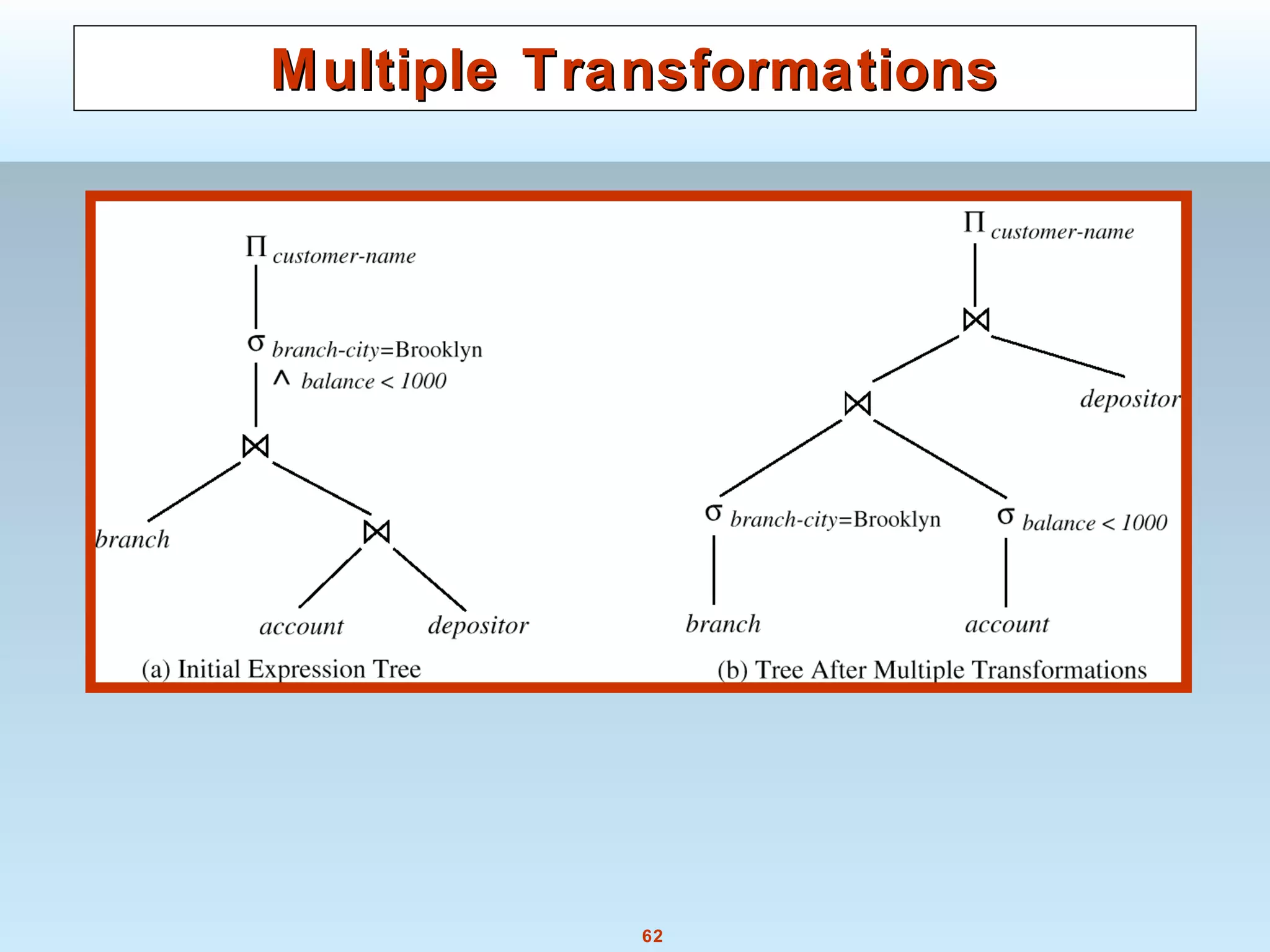
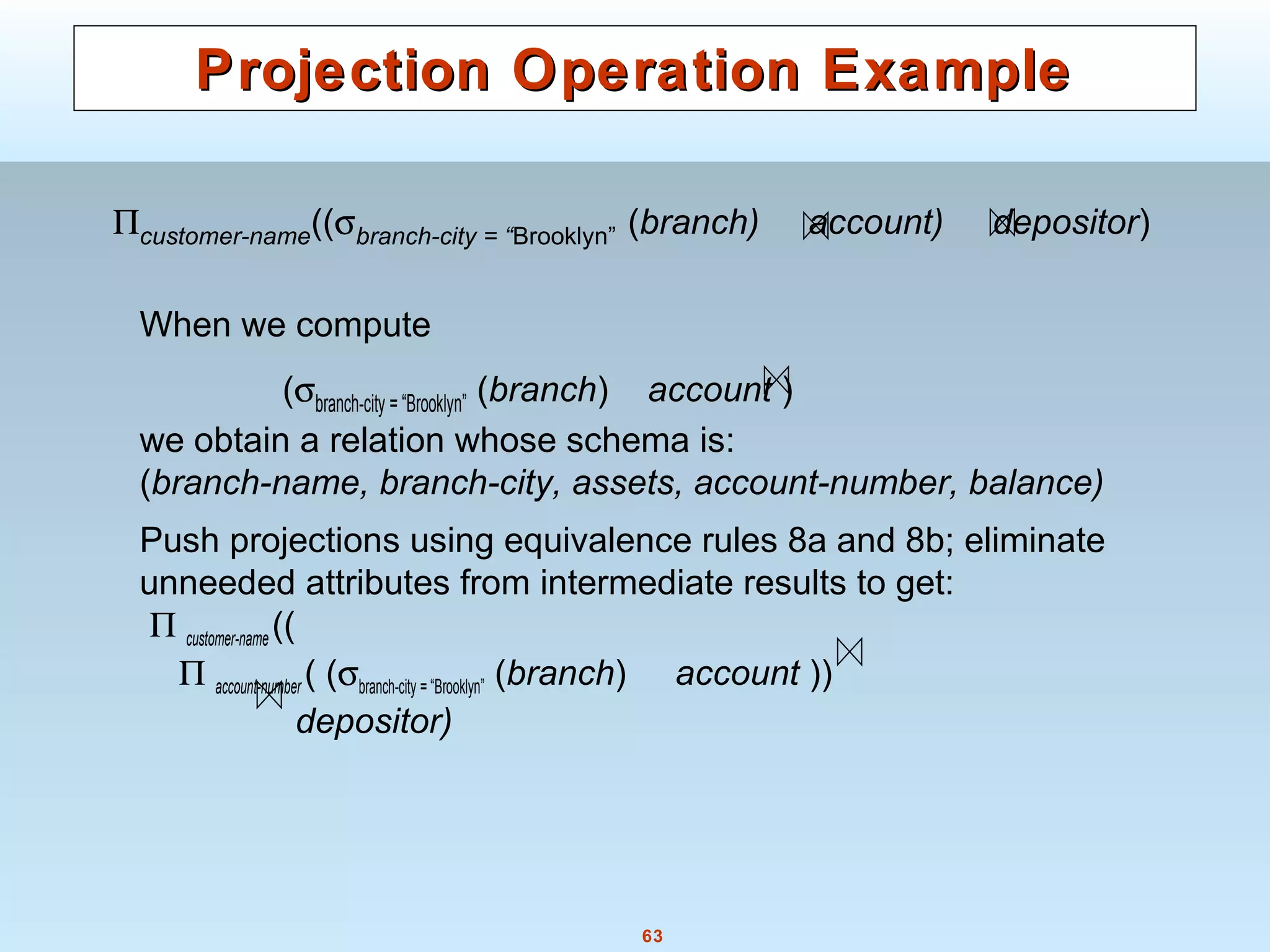
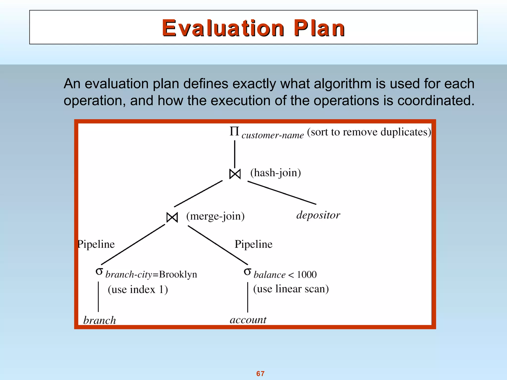
The document discusses various steps and algorithms involved in query processing in a database system. It covers parsing and translating a query, optimizing the query plan, and evaluating the query. Key operations discussed include selection, sorting, and join. For each operation, multiple algorithms are presented and their costs are analyzed based on factors like disk accesses and memory usage.


![[DSC Europe 25] Jim Sterne - Adopting Generative AI Capabilities Into the Ent...](https://cdn.slidesharecdn.com/ss_thumbnails/sxhpofuorcagxsaulkmt-3-251204082258-7e66bc48-thumbnail.jpg?width=640&height=640&fit=bounds)

![[DSC Europe 25] Dusan Jovicic - AI Story: From on-prem to cloud and back agai...](https://cdn.slidesharecdn.com/ss_thumbnails/8kp49m6uq22ifnbwhfnk-2-251205085715-964d11a6-thumbnail.jpg?width=640&height=640&fit=bounds)


![[DSC Europe 25] Nikola Rajovic - Hardware Technologies Under the Hood: RISC-V...](https://cdn.slidesharecdn.com/ss_thumbnails/o2gptrmtoyqndgoshwgq-dsc2025-tenstorrent-rajovic-251205090438-814685f5-thumbnail.jpg?width=640&height=640&fit=bounds)


![[DSC Europe 25] Dragan Vucic - Building the Learning Organization - How AI Tr...](https://cdn.slidesharecdn.com/ss_thumbnails/8brigo2sbu6qur6gxrra-7-251205085715-6ae07d24-thumbnail.jpg?width=640&height=640&fit=bounds)

![[DSC Europe 25] Andy Cotgreave - Nothing is new in analytics.pptx](https://cdn.slidesharecdn.com/ss_thumbnails/mba4vzcurvoh5lfrd5zw-6-251205194645-341bbbbe-thumbnail.jpg?width=640&height=640&fit=bounds)
![[DSC Europe 25] Goran Obradovic - The Rise of Sovereign AI: Building the Regi...](https://cdn.slidesharecdn.com/ss_thumbnails/7nw2xxixrxqdxvrb5wca-6-251205085714-ab09a2ac-thumbnail.jpg?width=640&height=640&fit=bounds)

