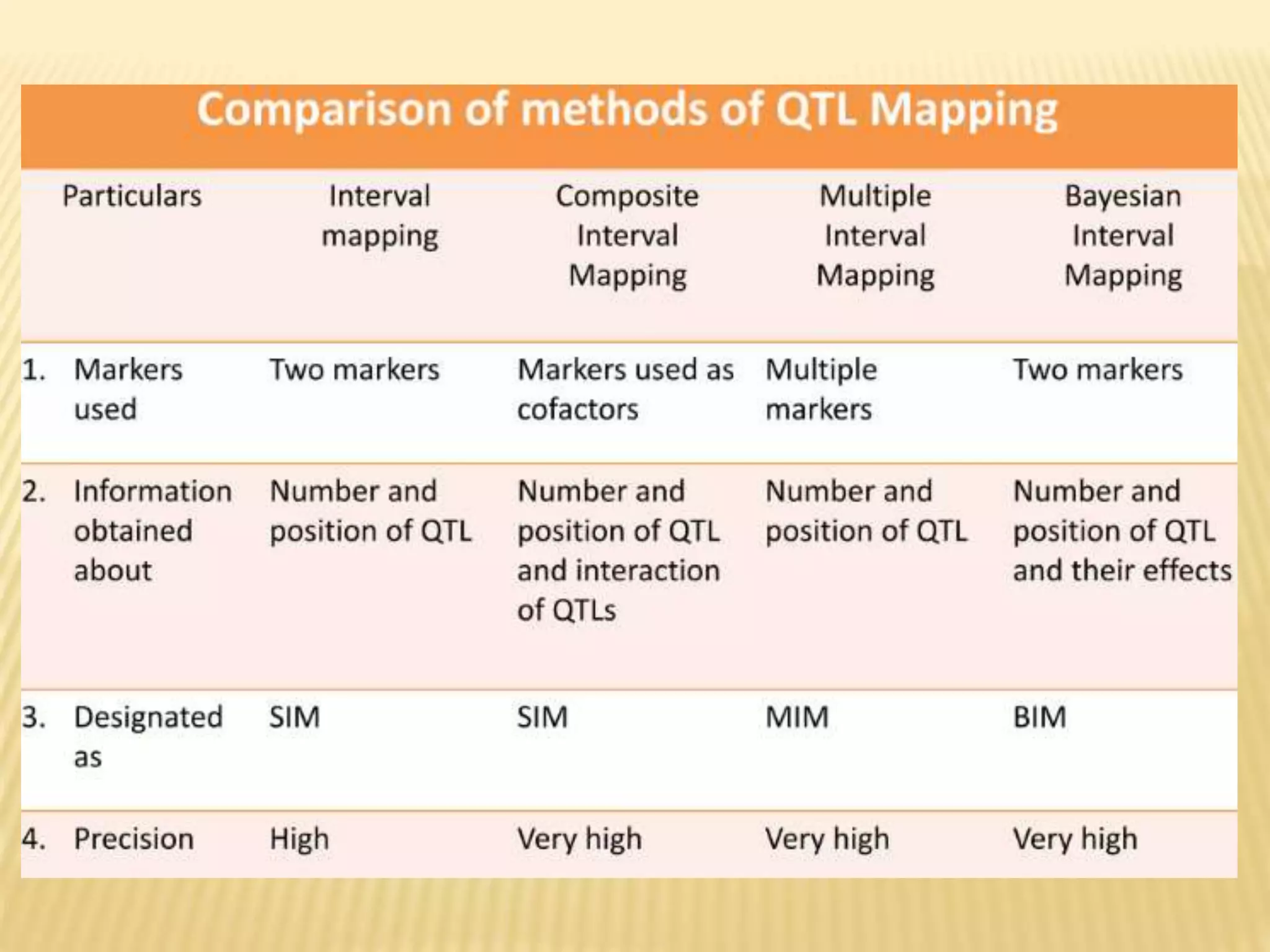
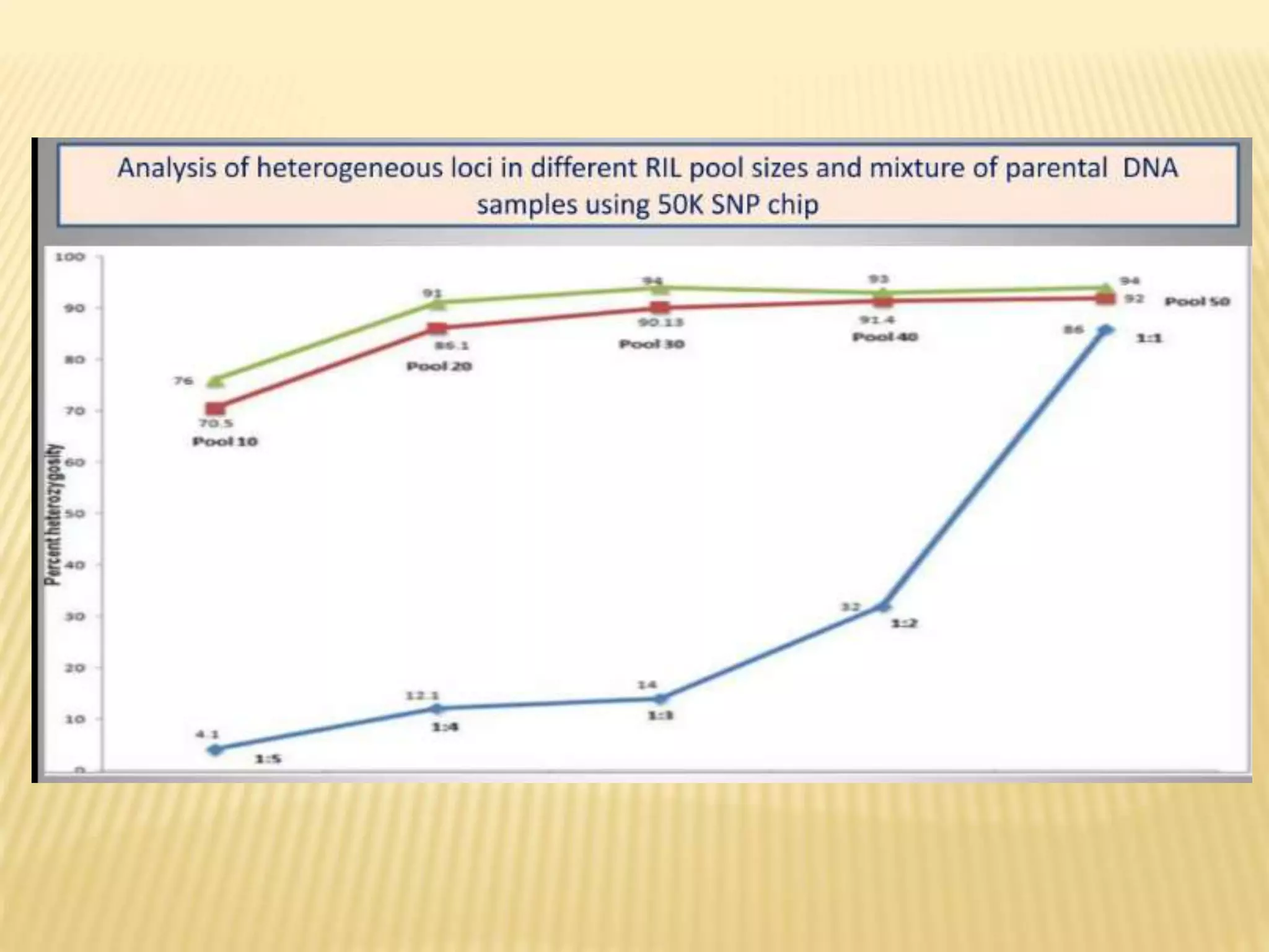
Topic : QTL MAPPING
Course Code- GPB 605
COURSE TITE- GENOMICS IN PLANT BREEDING
Presented to:
Dr.BAUDH BHARTI
Presentad by:
Prabhat Kumar Singh
Ph.D 1st Year 2nd Semester
QUANTITATIVE TRAIT LOCI
 The loci controlling quantitative traits are called quantitative trait loci
or QTL
 Term first coined by Gelderman in 1975.
 It is the region of the genome that is associated with an effect on a
quantitative trait.
 It can be a single gene or cluster of linked genes that affect the trait.
 A quantitative trait locus (QTL) is a position in a chromosome that
contains one or more polygenes involved in the determination of a
quantitative trait.
 The theory of QTL mapping was first described in 1923 by Sax; it was
noted that seed size in bean (a complex trait) was associated with seed
coat color (a monogenic trait).
QTLs have the following characteristics.
 These traits are controlled by multiple genes, each
segregating according to Mendel's laws.
 These traits can also be affected by the environment to
varying degrees.
 Many genes control any given trait and Allelic variations are
fully functional.
 Individual gene effects is small & The genes involved can be
dominant, or co- dominant.
 The genes involved can be subject to epistasis or
pleiotrophic effect
QTL Mapping
• The process of constructing linkage maps and conducting QTL
analysis i.e. to identify genomic regions associated with traits is
known as QTL mapping.
• Identification and location of polygenes or QTL by use of DNA
markers.
• It involves testing DNA markers throughout the genome for the
likelihood that they are associated with a QTL.
Principles of QTL mapping
• Genes and markers segregate via chromosome recombination
during meiosis, thus allowing their analysis in the progeny.
• The detection of association between phenotype and genotype of
markers.
• QTL analysis depends on the linkage disequilibrium.
• QTL analysis is usually undertaken in segregating mapping
populations
Objectives of QTL Mapping
The basic objective is to detect QTL, while minimizing the
occurrence of false positives (Type I errors, that is declaring an
association between a marker and QTL when in fact one does not
exist).
• To identify the regions of the genome that affects the trait of
interest.
• To analyze the effect of the QTL on the trait.
STEPS INVOLVED IN QTL MAPPING
 Selection of parental lines
 Sufficient polymorphism
 Parental lines are highly contrasting phenotypically
 Genetically divergent
 Selection of molecular markers (dominant/codominant)
 Making crosses
 Creation of mapping population
 Genotyping of the progenies
 Phenotyping of the progenies
 Construction of linkage map
 Screening the mapping population using polymorphic molecular
markers
 Segregation patterns
 Data is then analyzed using a statistical package such as
MAPMAKER or JOINMAP
 Assigning them to their linkage groups on the basis of
recombination values
 For practical purposes, in general recombination events
considered to be less than 10 recombinations per 100 meiosis, or
a map distance of less than 10 centiMorgans(cM).
METHODS TO DETECT QTLS
 Single-marker analysis
 Simple interval mapping
 Composite interval mapping
 Multiple Interval Mapping
 Bayesian Interval Mapping
SINGLE-MARKER ANALYSIS (SMA)
 Also known as single- point analysis. It is the simplest
method for detecting QTLs associated with single
markers
 This method does not require a complete linkage map
and can be performed with basic statistical software
programs.
 The statistical methods used for single-marker analysis
include t-tests, analysis of variance (ANOVA) and
linear regression.
 Linear regression is most commonly used because the
coefficient of determination (R2) from the marker
explains the phenotypic variation arising from the QTL
linked to the marker.
LIMITATIONS
 Likelihood of QTL detection significantly decreases as the
distance between the marker and QTL increases.
 It cannot determine whether the markers are associated with
one or more markers QTLs.
 The effects of QTL are likely to be underestimated because
they are confounded with recombination frequencies.
 To overcome these limitations the use of large number of
segregating DNA markers covering the entire genome may
minimize these problems.
 QGene and MapManager QTX are commonly used computer
programs to perform single- marker analysis
SIMPLE INTERVAL MAPPING (SIM)
.
 It was first proposed by Lander and Bolstein.
 It takes full advantages of the linkage map.
 This method evaluates the target association between the trait
values and the genotype of a hypothetical QTL (target QTL) at
multiple analysis points between pair of adjacent marker loci
(target interval).
 MapMaker/QTL and QGene are used to conduct SIM.
 The principle behind interval mapping is to test a model for the
presence of a QTL at many positions between two mapped loci.
LOGARITHM OF THE ODDS RATIO (LOD SCORE)
 Linkage between markers is usually calculated using odds
ratio.
 This ratio is more conveniently expressed as the logarithm of
the ratio, and is called a logarithm of odds (LOD) value or
LOD score.
 LOD values of >3 are typically used to construct linkage
maps.
 LOD of 2 means that it is 100 times more likely that a QTL
exists in the interval than that there is no QTL.
 LOD of 3 between two markers indicates that linkage is 1000
times more likely (i.e. 1000:1) than no linkage.
 LOD values may be lowered in order to detect a greater level of
linkage or to place additional markers within maps constructed at
higher LOD values.
The LOD score is a measure of the strength of evidence for the
presence of a QTL at a particular location.
 Hypothetical output showing a LOD profile for chromosome 4. The
dotted line represents the significance threshold determined by
permutation tests. The output indicates that the most likely position
for the QTL is near marker Q (indicated by an arrow). The best
flanking markers for this QTL would be Q and R.
Interval Mapping by Regression
 It is essentially the same as the method of basic QTL analysis
(regression on coded marker genotypes) except that phenotypes
are regressed on QTL genotypes.
 Since QTL genotypes are unknown they are replaced by
probabilities estimated from the nearest flanking markers.
 Softwares used: PLABQTL,QTL Cartographer, MapQTL
COMPOSITE INTERVAL MAPPING (CIM)
 Developed by Jansen and Stam in 1994
 It combines interval mapping for a single QTL in a given
interval with multiple regression analysis on marker
associated with other QTL.
 It is more precise and effective when linked QTLs are
involved.
 It considers marker interval plus a few other well chosen
single markers in each analysis, so that n-1 tests for
interval - QTL associations are performed on a
chromosome with n markers
ADVANTAGES
 Mapping of multiple QTLs can be accomplished by the
search in one dimension.
 By using linked markers as cofactors, the test is not
affected by QTL outside the region, thereby increasing
the precision of QTL mapping.
 By eliminating much of the genetic variance by other
QTL, the residual variance is reduced, thereby increasing
the power of detection of QTL.
Problems
 The effects of additional QTL will contribute to sampling
variation. If two QTL are linked their combined effects
will cause biased estimates.
MULTIPLE INTERVAL MAPPING (MIM)
 It is also a modification of simple interval mapping.
 It utilizes multiple marker intervals simultaneously to fit
multiple putative QTL directly in the model for mapping
QTL.
 It provides information about number and position of
QTL in the genome.
 It also determines interaction of significant QTLs and
their contribution to the genetic variance.
 It is based on Cockerham's model for interpreting genetic
parameters.
BAYESIAN INTERVAL MAPPING (BIM)
 It provides a model for QTL mapping
 It provides information about number and position of
QTL and their effects
 The BIM estimates should agree with MIM estimates
and should be similar to CIM estimates.
 It provides information posterior estimates of multiple
QTL in the intervals.
 It can estimate QTL effect and position separately
MERITS OF QTL MAPPING
 Identification of novel genes
 Where mutant approaches fail to detect genes with
phenotypic functions, QTL mapping can help
 Good alternative when mutant screening is laborious
and expensive e.g circadium rhythm screens
 Can identify New functional alleles of known
function genes
 e.g. Flowering time QTL, EDI was the CRY2 gene
 Natural variation studies provide insight into the
origins of plant evolution
LIMITATIONS
 Mainly identifies loci with large effects
 Less strong ones can be hard to pursue.
 No. of QTLs detected, their position and effects are subjected to
statistical error.
 Small additive effects / epistatic loci are not detected and may
require further analyses.
Future Prospects
 Constant improvements of Molecular platforms
 New Types of genetic materials (e.g. introgression lines: small
effect QTLs can be detected)
 Advances in Bioinformatics
CASE STUDY
 MAPPING QTLS FOR SALT TOLERANCE IN RICE
(Oryza sativa L.)
 BY BULKED SEGREGANT ANALYSIS OF
RECOMBINANT INBRED LINES (RIL'S)
 Sushma Tiwari, et al JOURNAL:PLOS GENETICS
 NASS RATING:12.66
ABSTRACT
 Rapid identification of QTLs for reproductive stages tolerance using
bulked segregant analysis(BSA) of bi- parental recombinant inbred lines
(RIL).
 The parents and bulks were genotype using a 50K SNP chip to identify
genomic regions showing homogeneity for contrasting allele showing
polymorphic SNPs in the two bulks.
 The method was applied to 'CSR11/M148' RILS segregating for
reproductive stage salt tolerance. The method was validated further with
'CSR27/M148' RILS used earlier for mapping salt tolerance QTLs using
low density SSR markers.
 BSA with 50K SNP chip revealed 5,021 polymorphic loci and 34 QTL
regions. This not only confirmed the location of previously mapped
QTLs but also identified several new QTLs, and provided a rapid way to
scan the whole genome for mapping QTLs for complex agronomic traits
in rice.
MATERIALS AND METHODS
 A mapping population of 216 recombinant inbred lines
(RILS) was developed from across between rice varieties
CSR11 and MI48 using single seed descent method.
 Mapping QTLs for Salt Stress in Rice by BSA Using
50K SNP Chip.
RESULTS AND DISCUSSION
• Study out of 34 QTLs of CSR27/M148 population five QTLs
were reported earlier in the and found 29 novel QTL regions on
rice chromosomes 1,2,3,5,6,9,11 and 12 due to dense SNP map of
polymorphic locus covering all regions of the genome.
• Earlier highest 41 QTLs have been reported by Ghomi et al, on
all the 12 rice chromosomes for salinity tolerance at seedling stage
in rice.
• There are several reports on QTL mapping for salt stress by SSR
genotyping on whole population in rice but no one has done QTL
mapping by BSA approach for salt stress in rice. It gives clear
picture that QTL mapping effective in identification of tolerant
alleles.
REFERENCES
 Kearsey, M.J. and Pooni, H.S. 1996. The genetical
analysis of quantitative traits. Chapter 7
 Bernardo, R. 2002. Breeding for quantitative traits in
plants. Chapters 13 and 14

QTL MAPPING.pptx

  • 1.
    Topic : QTLMAPPING Course Code- GPB 605 COURSE TITE- GENOMICS IN PLANT BREEDING Presented to: Dr.BAUDH BHARTI Presentad by: Prabhat Kumar Singh Ph.D 1st Year 2nd Semester
  • 2.
    QUANTITATIVE TRAIT LOCI The loci controlling quantitative traits are called quantitative trait loci or QTL  Term first coined by Gelderman in 1975.  It is the region of the genome that is associated with an effect on a quantitative trait.  It can be a single gene or cluster of linked genes that affect the trait.  A quantitative trait locus (QTL) is a position in a chromosome that contains one or more polygenes involved in the determination of a quantitative trait.  The theory of QTL mapping was first described in 1923 by Sax; it was noted that seed size in bean (a complex trait) was associated with seed coat color (a monogenic trait).
  • 3.
    QTLs have thefollowing characteristics.  These traits are controlled by multiple genes, each segregating according to Mendel's laws.  These traits can also be affected by the environment to varying degrees.  Many genes control any given trait and Allelic variations are fully functional.  Individual gene effects is small & The genes involved can be dominant, or co- dominant.  The genes involved can be subject to epistasis or pleiotrophic effect
  • 4.
    QTL Mapping • Theprocess of constructing linkage maps and conducting QTL analysis i.e. to identify genomic regions associated with traits is known as QTL mapping. • Identification and location of polygenes or QTL by use of DNA markers. • It involves testing DNA markers throughout the genome for the likelihood that they are associated with a QTL. Principles of QTL mapping • Genes and markers segregate via chromosome recombination during meiosis, thus allowing their analysis in the progeny. • The detection of association between phenotype and genotype of markers. • QTL analysis depends on the linkage disequilibrium. • QTL analysis is usually undertaken in segregating mapping populations
  • 5.
    Objectives of QTLMapping The basic objective is to detect QTL, while minimizing the occurrence of false positives (Type I errors, that is declaring an association between a marker and QTL when in fact one does not exist). • To identify the regions of the genome that affects the trait of interest. • To analyze the effect of the QTL on the trait.
  • 6.
    STEPS INVOLVED INQTL MAPPING  Selection of parental lines  Sufficient polymorphism  Parental lines are highly contrasting phenotypically  Genetically divergent  Selection of molecular markers (dominant/codominant)  Making crosses  Creation of mapping population
  • 7.
     Genotyping ofthe progenies  Phenotyping of the progenies  Construction of linkage map  Screening the mapping population using polymorphic molecular markers  Segregation patterns  Data is then analyzed using a statistical package such as MAPMAKER or JOINMAP  Assigning them to their linkage groups on the basis of recombination values  For practical purposes, in general recombination events considered to be less than 10 recombinations per 100 meiosis, or a map distance of less than 10 centiMorgans(cM).
  • 8.
    METHODS TO DETECTQTLS  Single-marker analysis  Simple interval mapping  Composite interval mapping  Multiple Interval Mapping  Bayesian Interval Mapping
  • 9.
    SINGLE-MARKER ANALYSIS (SMA) Also known as single- point analysis. It is the simplest method for detecting QTLs associated with single markers  This method does not require a complete linkage map and can be performed with basic statistical software programs.  The statistical methods used for single-marker analysis include t-tests, analysis of variance (ANOVA) and linear regression.  Linear regression is most commonly used because the coefficient of determination (R2) from the marker explains the phenotypic variation arising from the QTL linked to the marker.
  • 10.
    LIMITATIONS  Likelihood ofQTL detection significantly decreases as the distance between the marker and QTL increases.  It cannot determine whether the markers are associated with one or more markers QTLs.  The effects of QTL are likely to be underestimated because they are confounded with recombination frequencies.  To overcome these limitations the use of large number of segregating DNA markers covering the entire genome may minimize these problems.  QGene and MapManager QTX are commonly used computer programs to perform single- marker analysis
  • 11.
    SIMPLE INTERVAL MAPPING(SIM) .  It was first proposed by Lander and Bolstein.  It takes full advantages of the linkage map.  This method evaluates the target association between the trait values and the genotype of a hypothetical QTL (target QTL) at multiple analysis points between pair of adjacent marker loci (target interval).  MapMaker/QTL and QGene are used to conduct SIM.  The principle behind interval mapping is to test a model for the presence of a QTL at many positions between two mapped loci.
  • 12.
    LOGARITHM OF THEODDS RATIO (LOD SCORE)  Linkage between markers is usually calculated using odds ratio.  This ratio is more conveniently expressed as the logarithm of the ratio, and is called a logarithm of odds (LOD) value or LOD score.  LOD values of >3 are typically used to construct linkage maps.  LOD of 2 means that it is 100 times more likely that a QTL exists in the interval than that there is no QTL.
  • 13.
     LOD of3 between two markers indicates that linkage is 1000 times more likely (i.e. 1000:1) than no linkage.  LOD values may be lowered in order to detect a greater level of linkage or to place additional markers within maps constructed at higher LOD values. The LOD score is a measure of the strength of evidence for the presence of a QTL at a particular location.
  • 14.
     Hypothetical outputshowing a LOD profile for chromosome 4. The dotted line represents the significance threshold determined by permutation tests. The output indicates that the most likely position for the QTL is near marker Q (indicated by an arrow). The best flanking markers for this QTL would be Q and R. Interval Mapping by Regression  It is essentially the same as the method of basic QTL analysis (regression on coded marker genotypes) except that phenotypes are regressed on QTL genotypes.  Since QTL genotypes are unknown they are replaced by probabilities estimated from the nearest flanking markers.  Softwares used: PLABQTL,QTL Cartographer, MapQTL
  • 15.
    COMPOSITE INTERVAL MAPPING(CIM)  Developed by Jansen and Stam in 1994  It combines interval mapping for a single QTL in a given interval with multiple regression analysis on marker associated with other QTL.  It is more precise and effective when linked QTLs are involved.  It considers marker interval plus a few other well chosen single markers in each analysis, so that n-1 tests for interval - QTL associations are performed on a chromosome with n markers
  • 16.
    ADVANTAGES  Mapping ofmultiple QTLs can be accomplished by the search in one dimension.  By using linked markers as cofactors, the test is not affected by QTL outside the region, thereby increasing the precision of QTL mapping.  By eliminating much of the genetic variance by other QTL, the residual variance is reduced, thereby increasing the power of detection of QTL. Problems  The effects of additional QTL will contribute to sampling variation. If two QTL are linked their combined effects will cause biased estimates.
  • 17.
    MULTIPLE INTERVAL MAPPING(MIM)  It is also a modification of simple interval mapping.  It utilizes multiple marker intervals simultaneously to fit multiple putative QTL directly in the model for mapping QTL.  It provides information about number and position of QTL in the genome.  It also determines interaction of significant QTLs and their contribution to the genetic variance.  It is based on Cockerham's model for interpreting genetic parameters.
  • 18.
    BAYESIAN INTERVAL MAPPING(BIM)  It provides a model for QTL mapping  It provides information about number and position of QTL and their effects  The BIM estimates should agree with MIM estimates and should be similar to CIM estimates.  It provides information posterior estimates of multiple QTL in the intervals.  It can estimate QTL effect and position separately
  • 19.
    MERITS OF QTLMAPPING  Identification of novel genes  Where mutant approaches fail to detect genes with phenotypic functions, QTL mapping can help  Good alternative when mutant screening is laborious and expensive e.g circadium rhythm screens  Can identify New functional alleles of known function genes  e.g. Flowering time QTL, EDI was the CRY2 gene  Natural variation studies provide insight into the origins of plant evolution
  • 20.
    LIMITATIONS  Mainly identifiesloci with large effects  Less strong ones can be hard to pursue.  No. of QTLs detected, their position and effects are subjected to statistical error.  Small additive effects / epistatic loci are not detected and may require further analyses. Future Prospects  Constant improvements of Molecular platforms  New Types of genetic materials (e.g. introgression lines: small effect QTLs can be detected)  Advances in Bioinformatics
  • 22.
    CASE STUDY  MAPPINGQTLS FOR SALT TOLERANCE IN RICE (Oryza sativa L.)  BY BULKED SEGREGANT ANALYSIS OF RECOMBINANT INBRED LINES (RIL'S)  Sushma Tiwari, et al JOURNAL:PLOS GENETICS  NASS RATING:12.66
  • 23.
    ABSTRACT  Rapid identificationof QTLs for reproductive stages tolerance using bulked segregant analysis(BSA) of bi- parental recombinant inbred lines (RIL).  The parents and bulks were genotype using a 50K SNP chip to identify genomic regions showing homogeneity for contrasting allele showing polymorphic SNPs in the two bulks.  The method was applied to 'CSR11/M148' RILS segregating for reproductive stage salt tolerance. The method was validated further with 'CSR27/M148' RILS used earlier for mapping salt tolerance QTLs using low density SSR markers.  BSA with 50K SNP chip revealed 5,021 polymorphic loci and 34 QTL regions. This not only confirmed the location of previously mapped QTLs but also identified several new QTLs, and provided a rapid way to scan the whole genome for mapping QTLs for complex agronomic traits in rice.
  • 24.
    MATERIALS AND METHODS A mapping population of 216 recombinant inbred lines (RILS) was developed from across between rice varieties CSR11 and MI48 using single seed descent method.  Mapping QTLs for Salt Stress in Rice by BSA Using 50K SNP Chip.
  • 27.
    RESULTS AND DISCUSSION •Study out of 34 QTLs of CSR27/M148 population five QTLs were reported earlier in the and found 29 novel QTL regions on rice chromosomes 1,2,3,5,6,9,11 and 12 due to dense SNP map of polymorphic locus covering all regions of the genome. • Earlier highest 41 QTLs have been reported by Ghomi et al, on all the 12 rice chromosomes for salinity tolerance at seedling stage in rice. • There are several reports on QTL mapping for salt stress by SSR genotyping on whole population in rice but no one has done QTL mapping by BSA approach for salt stress in rice. It gives clear picture that QTL mapping effective in identification of tolerant alleles.
  • 28.
    REFERENCES  Kearsey, M.J.and Pooni, H.S. 1996. The genetical analysis of quantitative traits. Chapter 7  Bernardo, R. 2002. Breeding for quantitative traits in plants. Chapters 13 and 14