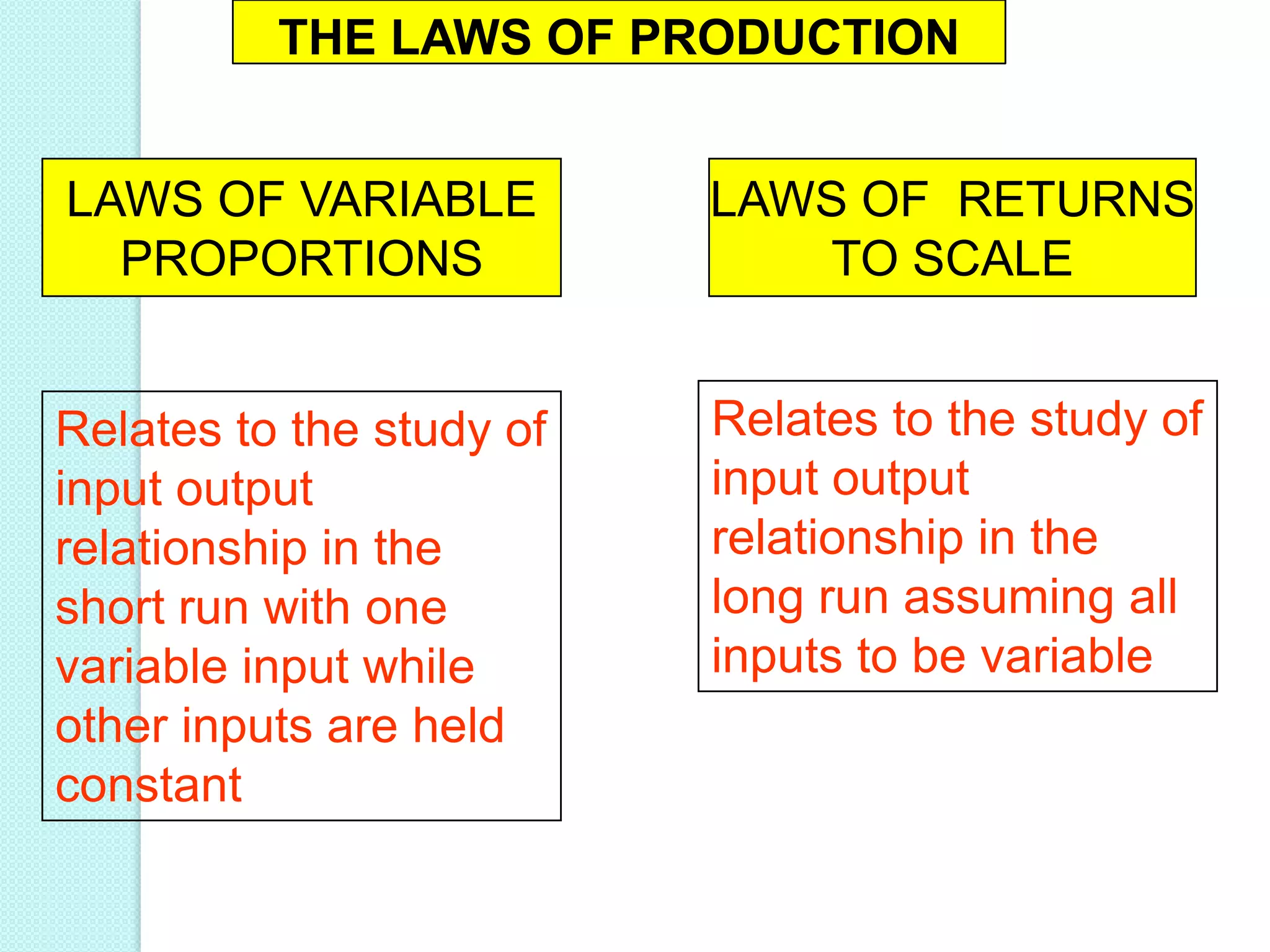
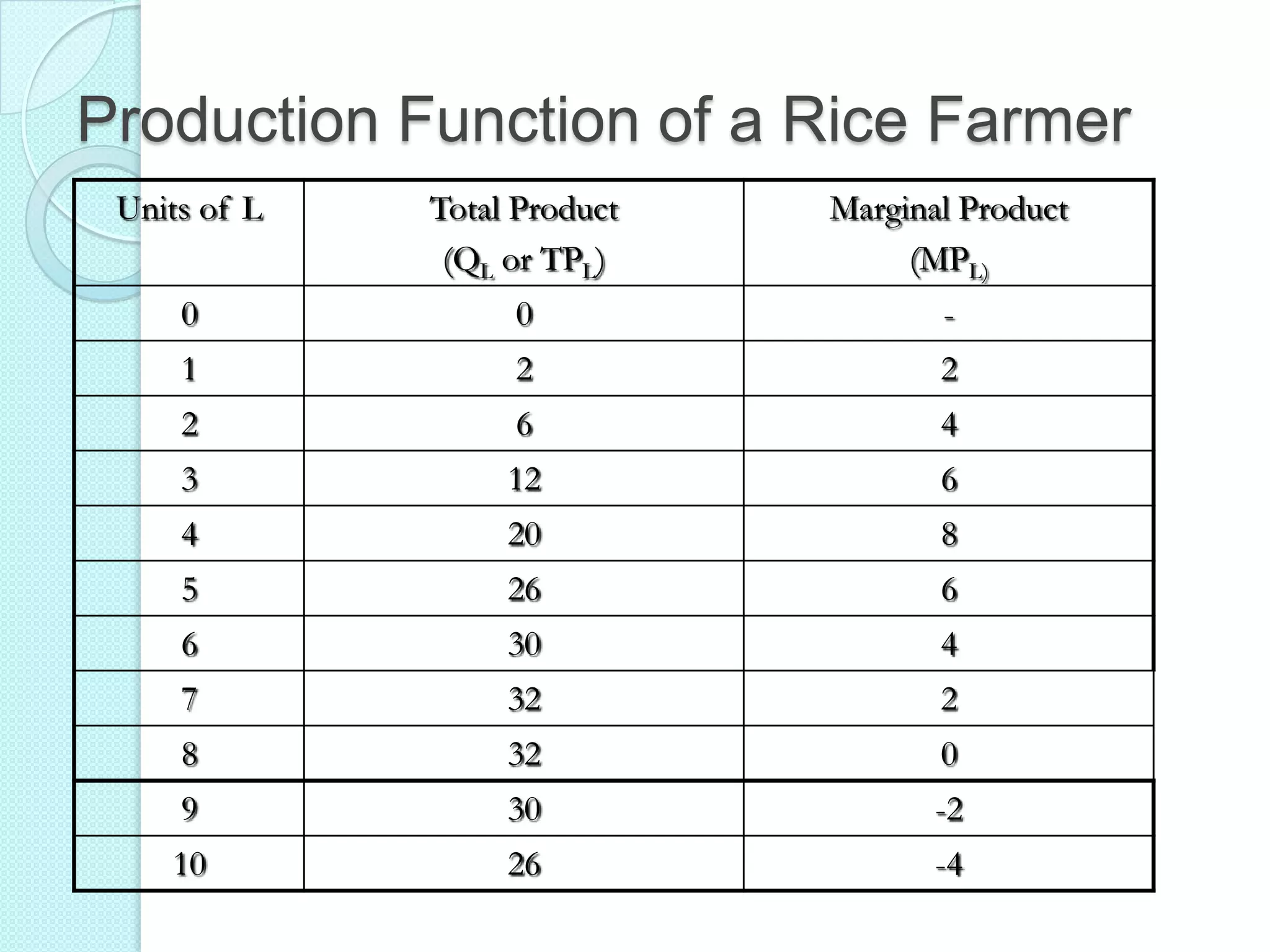
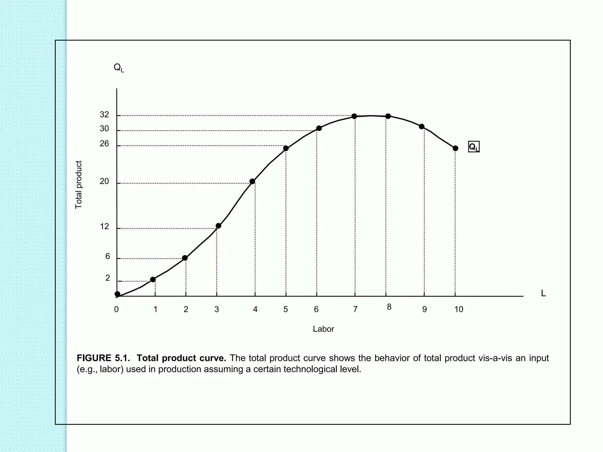
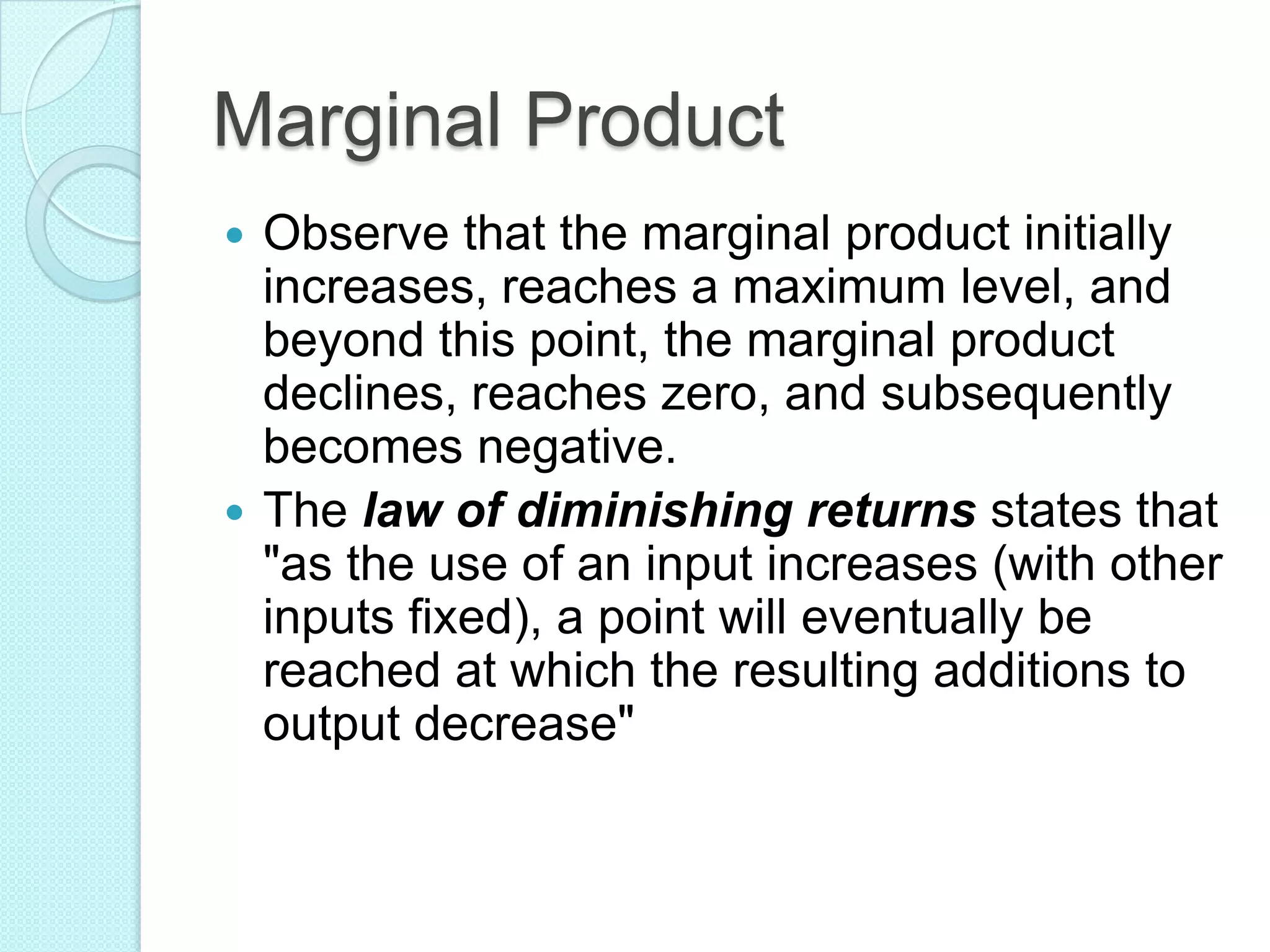
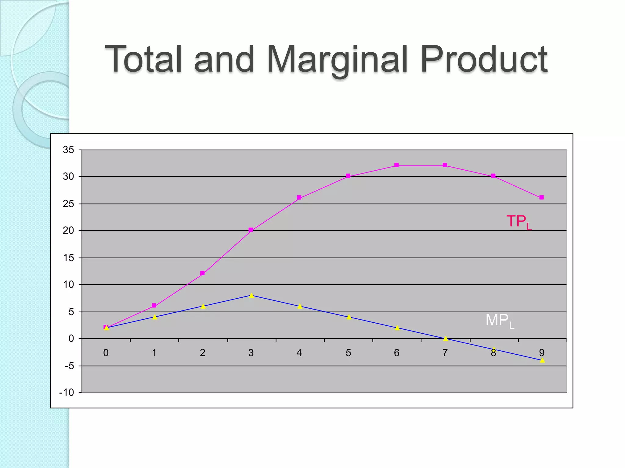
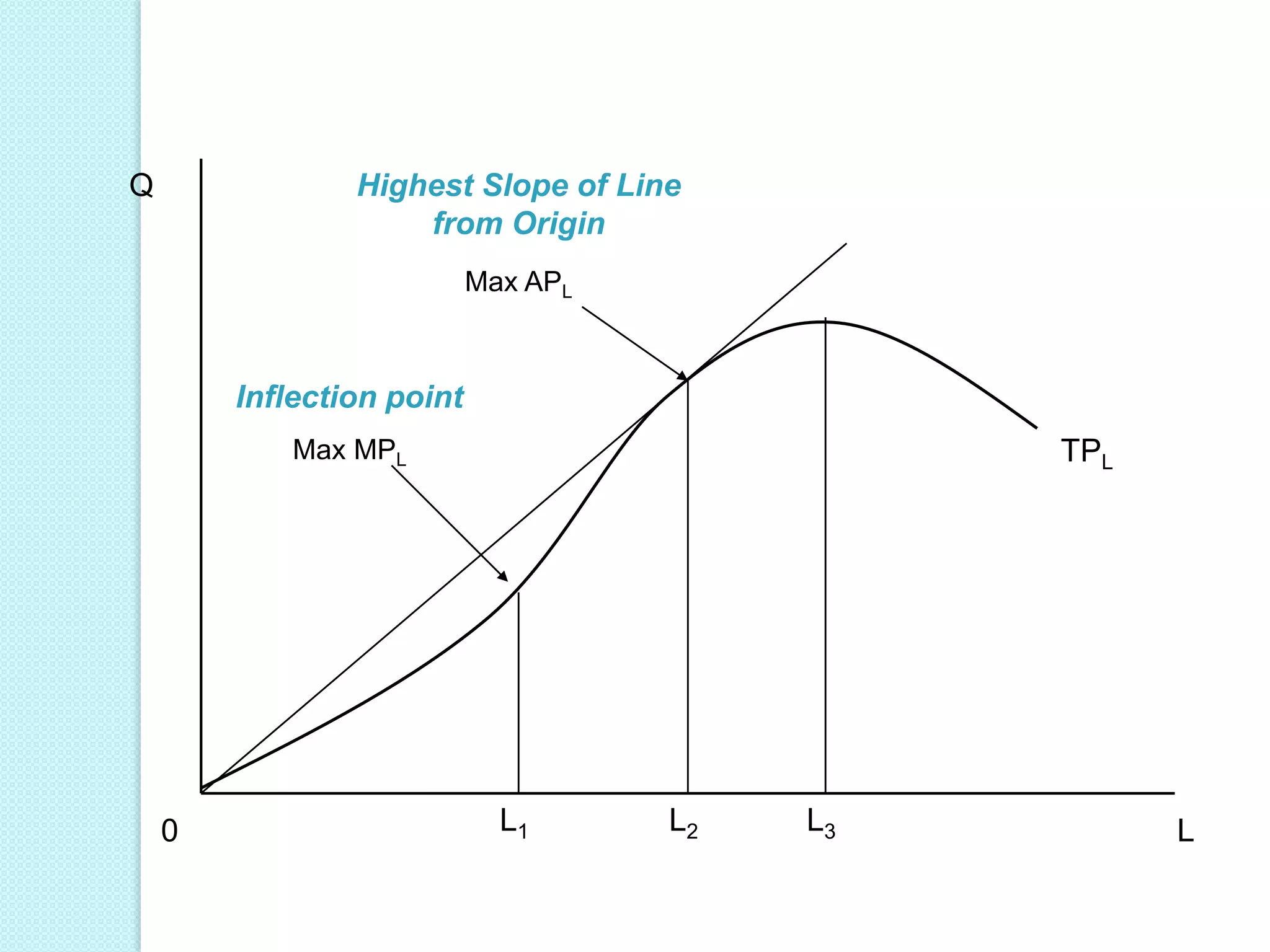
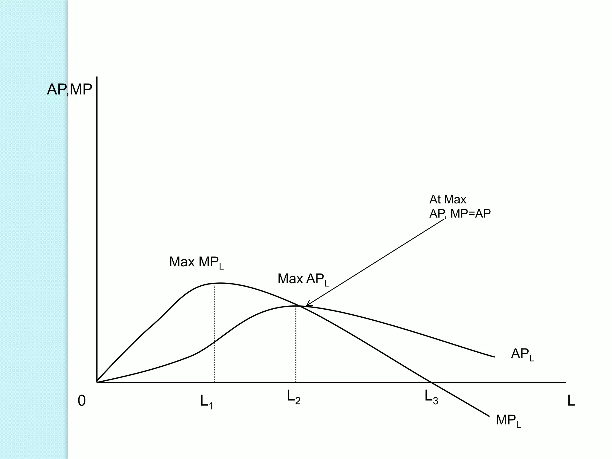
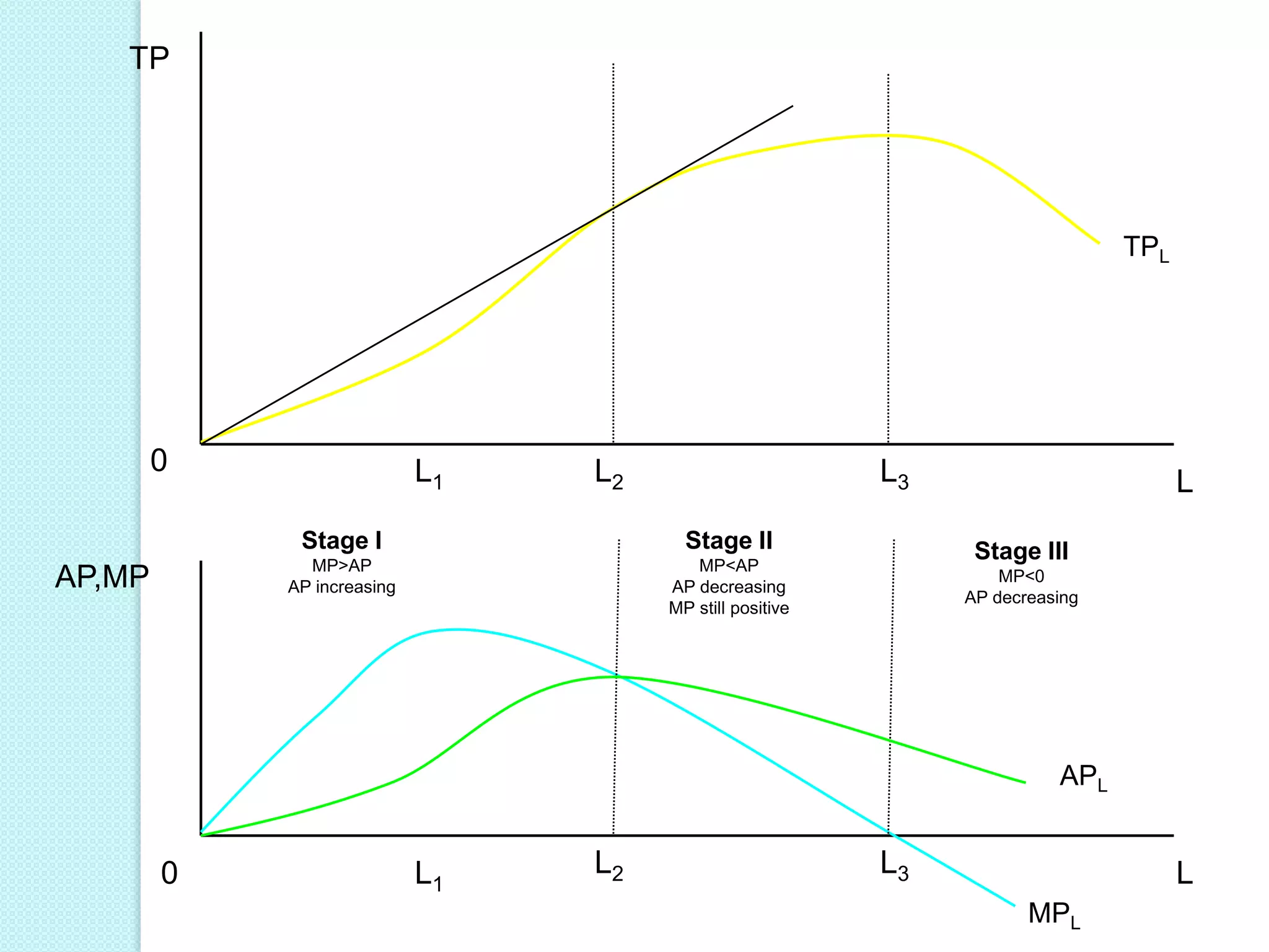
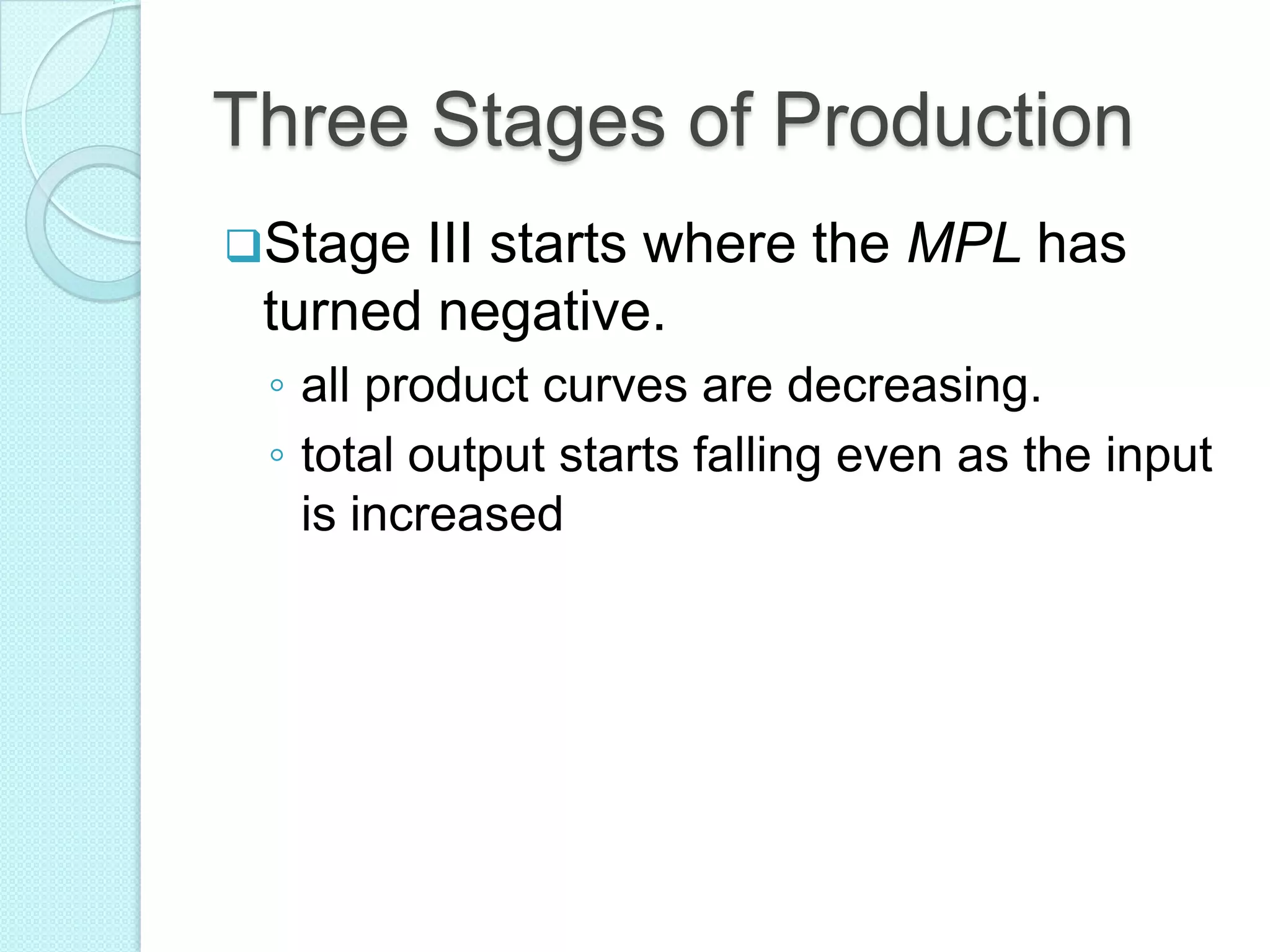
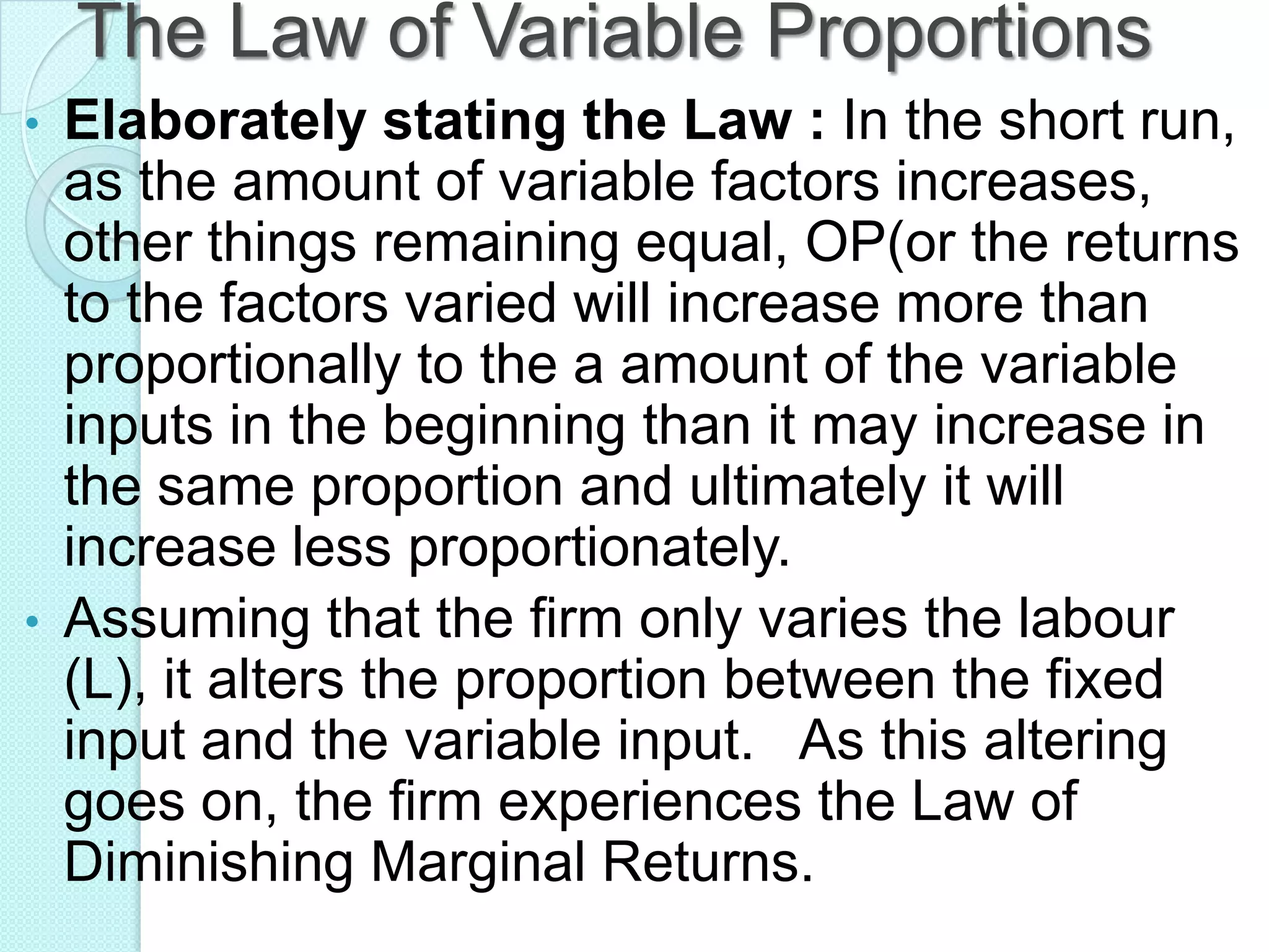
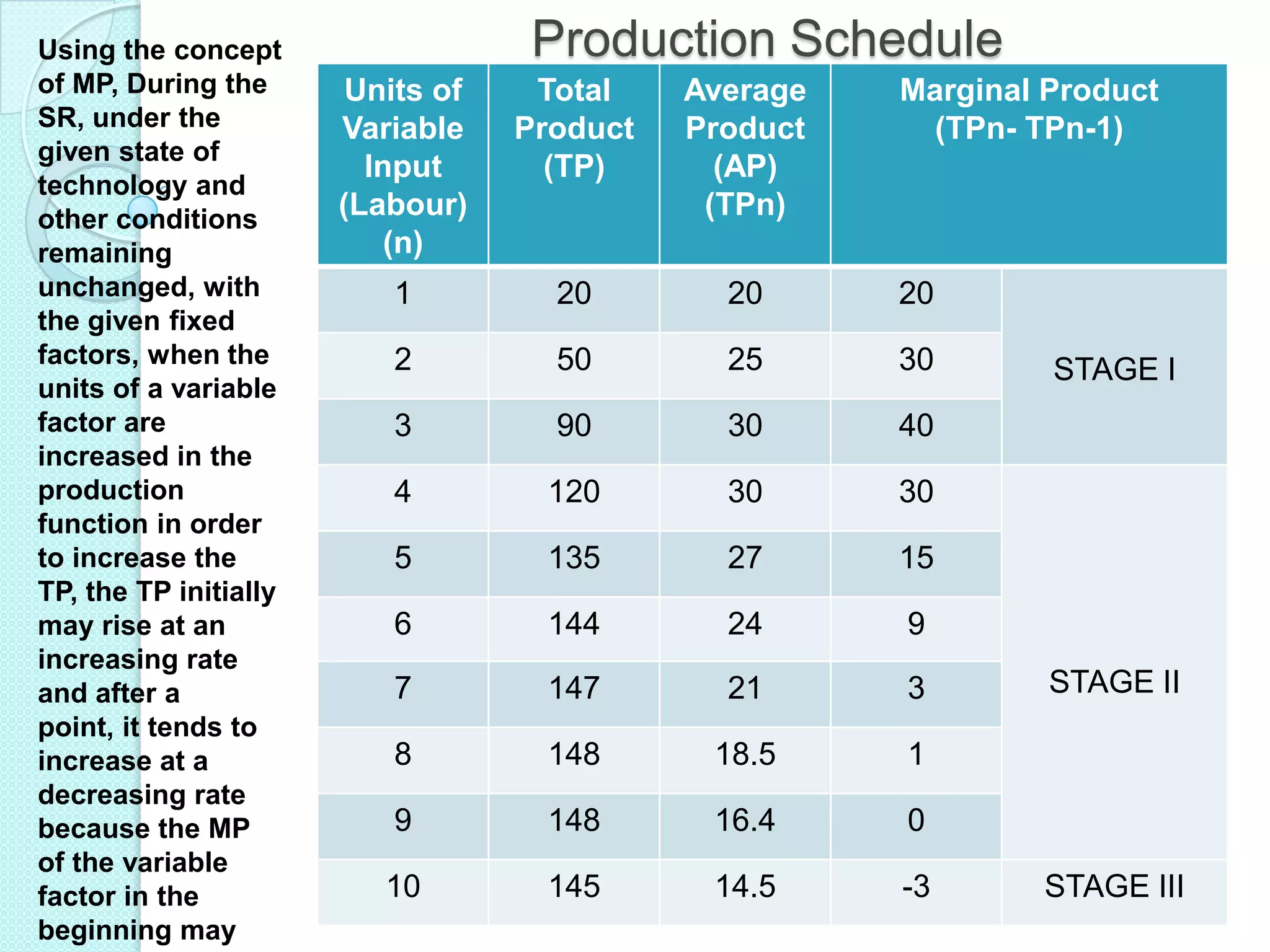
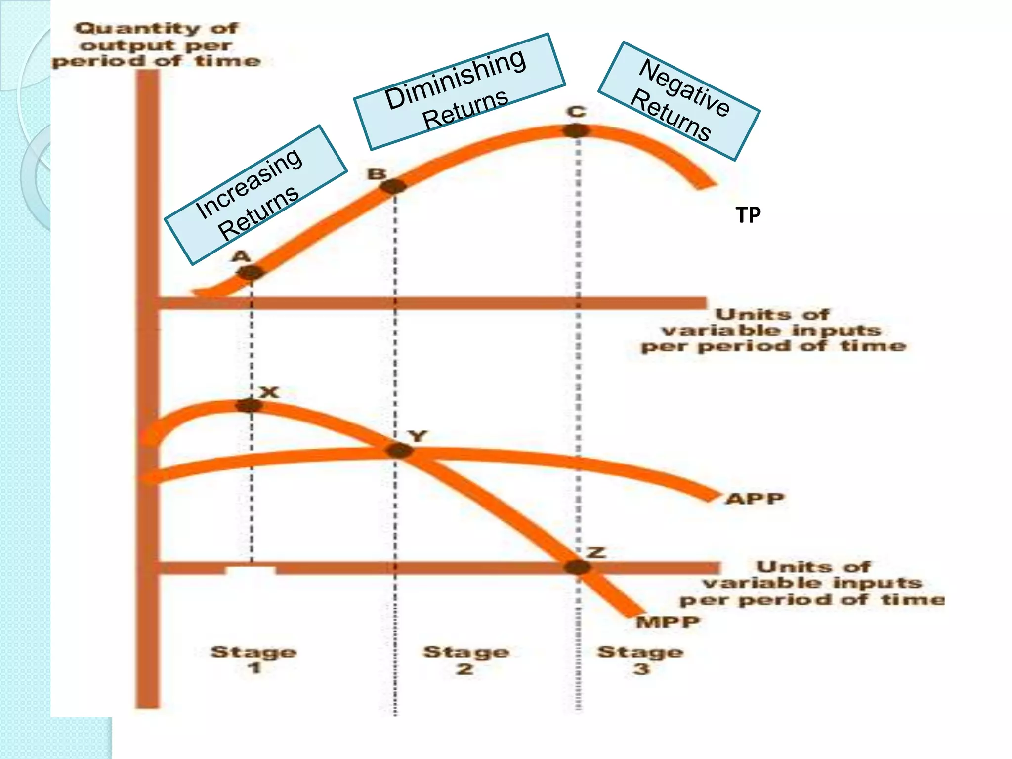
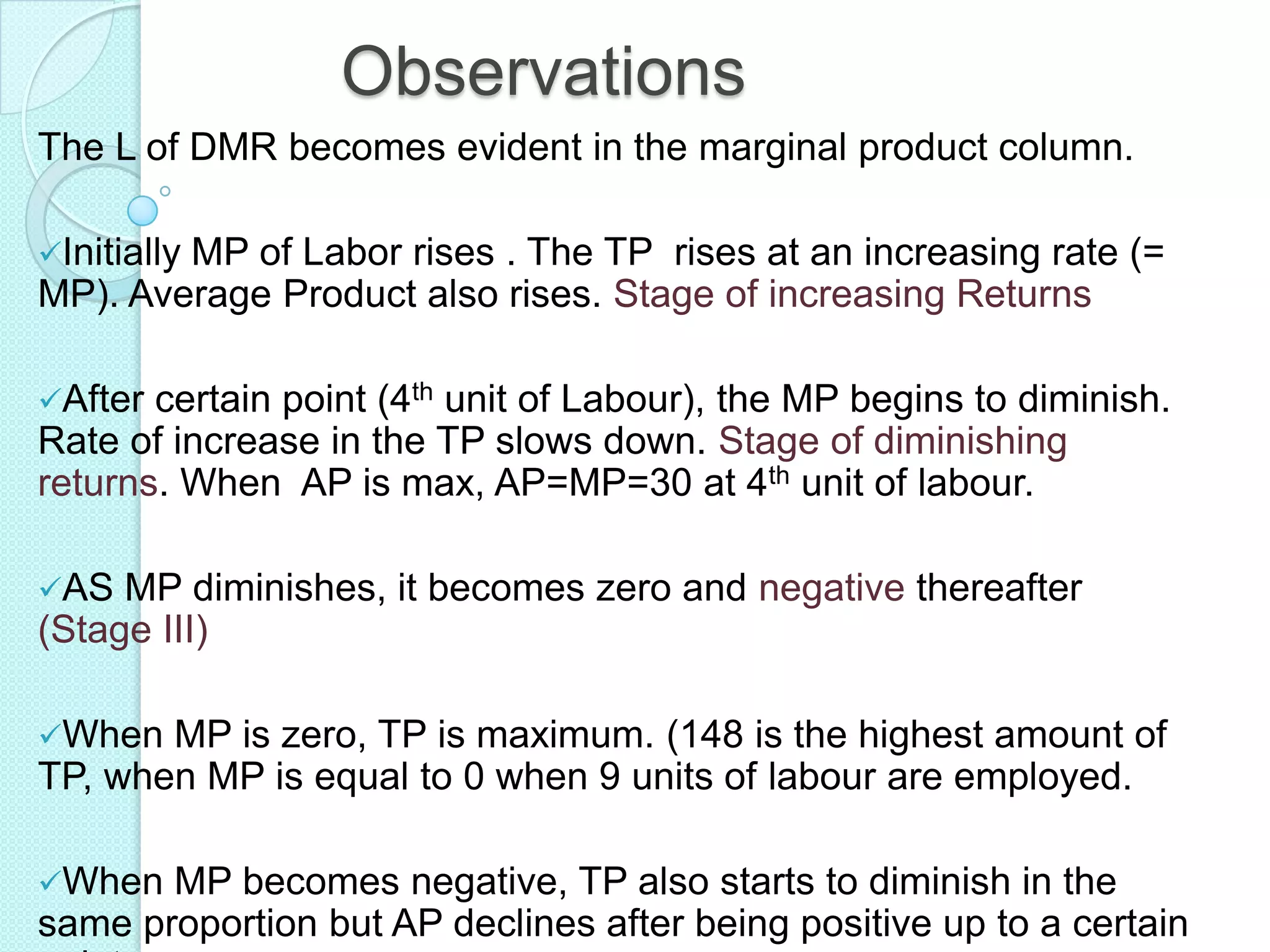
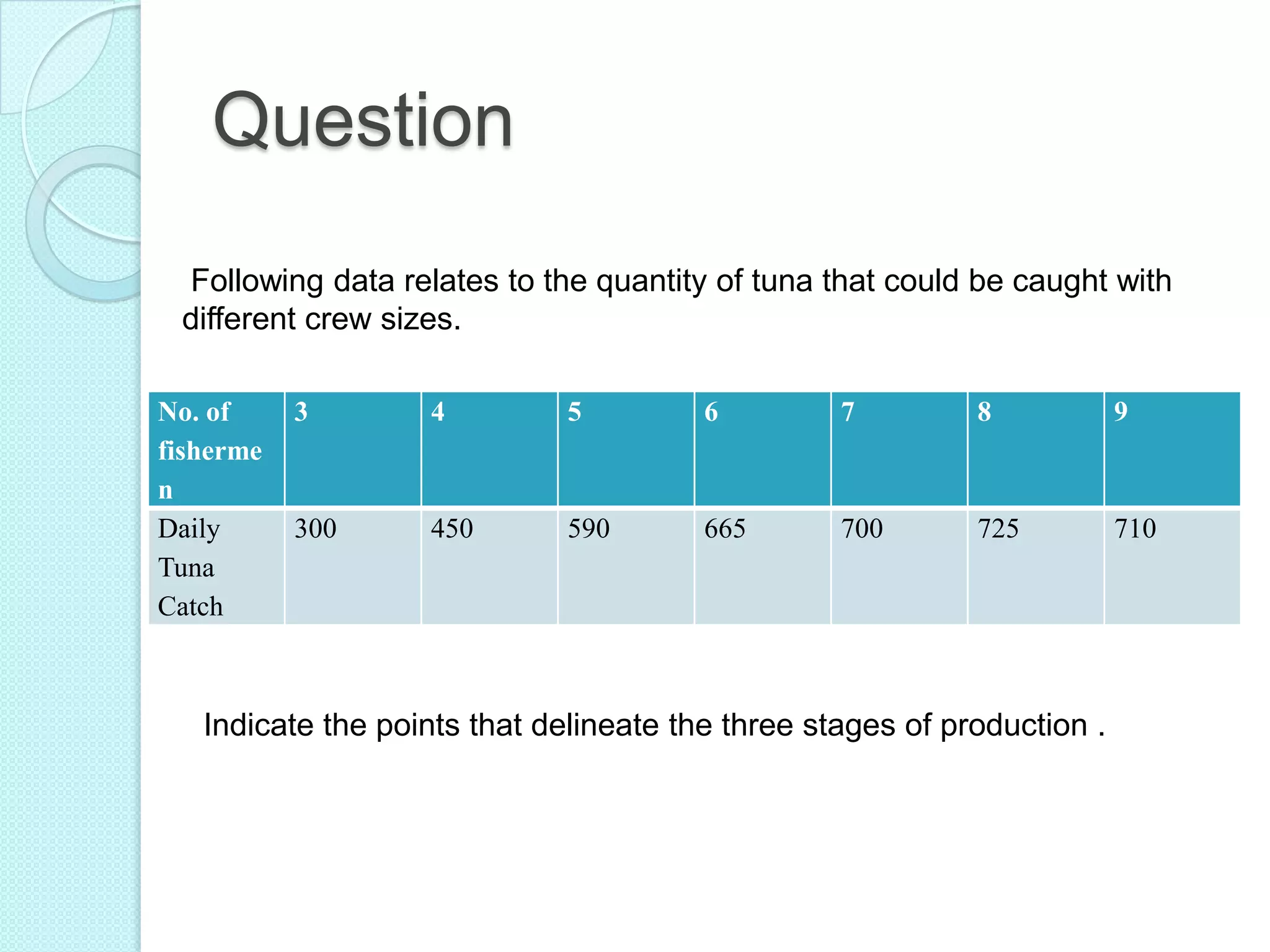
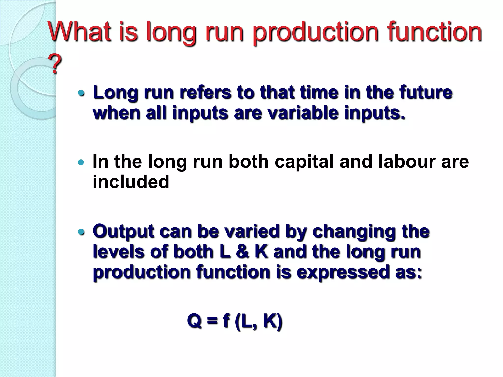
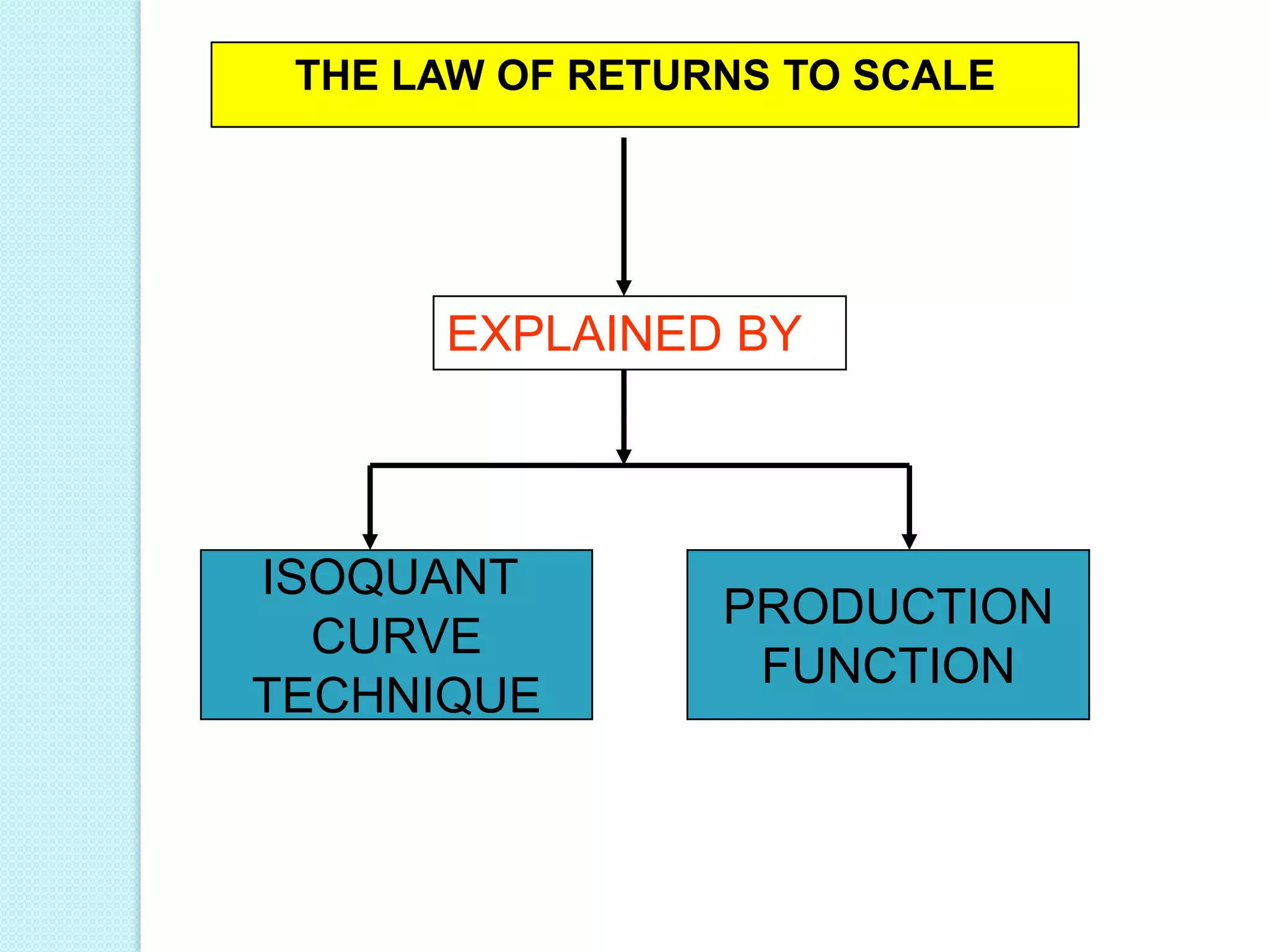
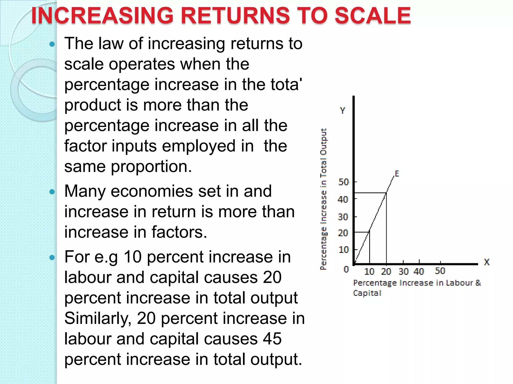
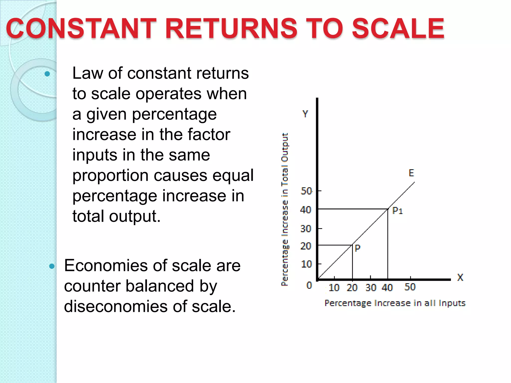
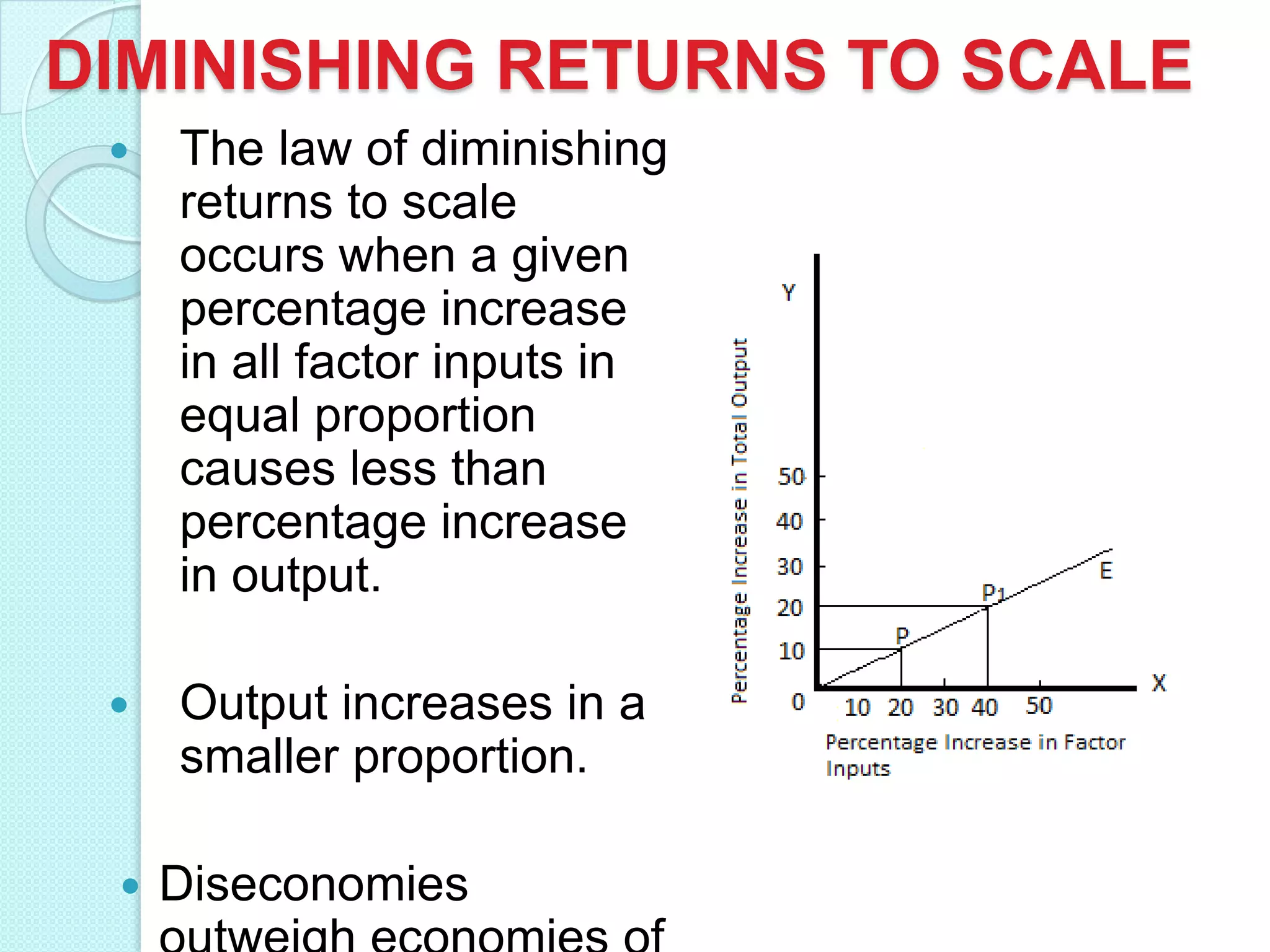
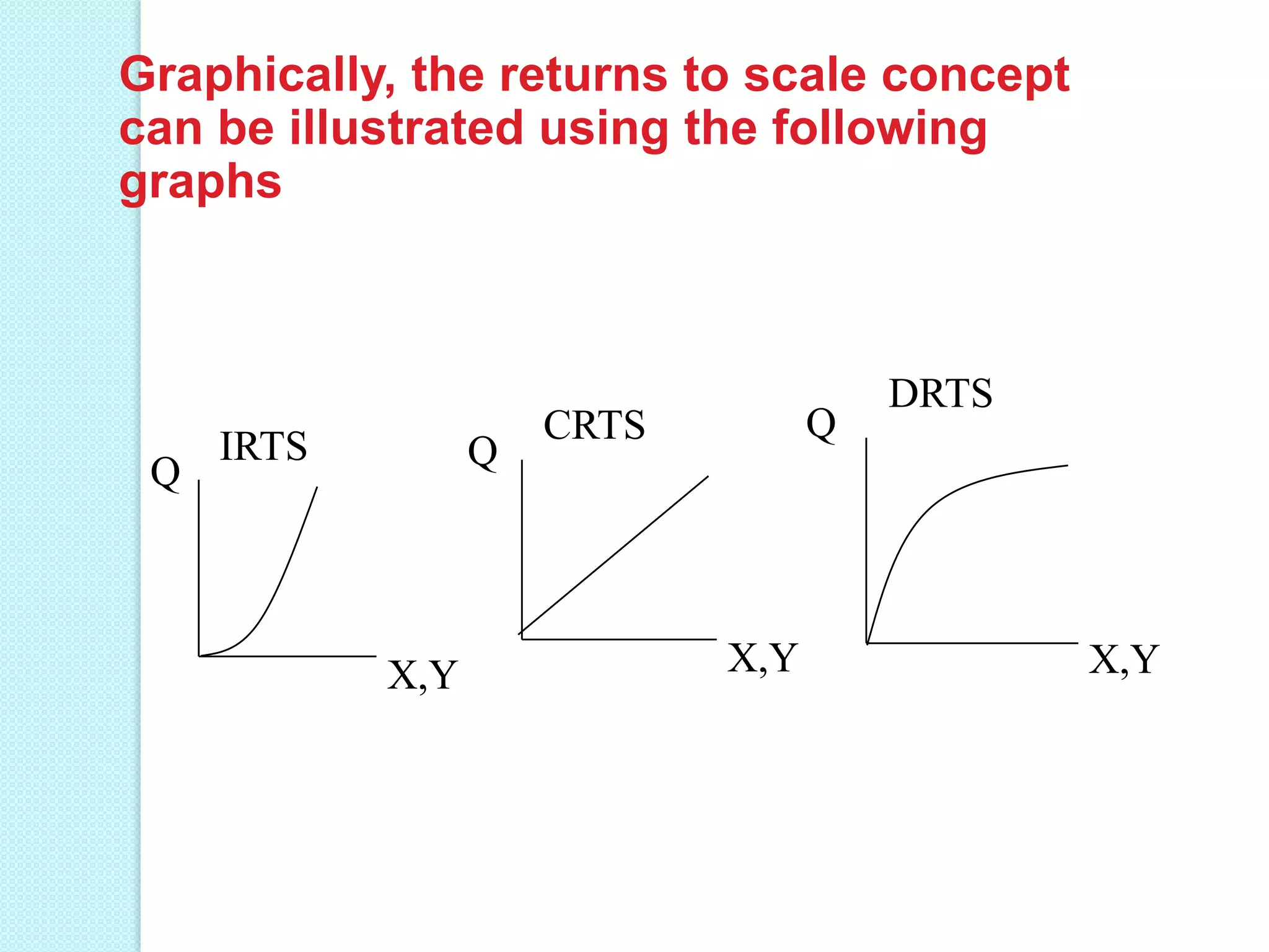
This document discusses production analysis and the theory of production costs from the perspective of a firm. It covers key concepts such as: - The three stages of production as defined by total, average, and marginal product curves. In stage one, average product is increasing. In stage two, average product is decreasing while marginal product turns negative in stage three. - Laws of variable proportions which state that as a variable input increases, total product initially increases at an increasing rate, then at a decreasing rate, due to diminishing marginal returns. - Long run production functions which consider all inputs as variable. Returns to scale can be increasing, constant, or diminishing based on how total output responds to a proportional increase

1. PRODUCTION ANALYSIS

2. Production

An entrepreneur must put together
resources -- land, labour, capital -- and
produce a product people will be
willing and able to purchase

3. Theory of Production and
Costs
Focus- mainly on the the firm.
 We will examine

◦ Its production capacity given available
resources
◦ the related costs involved

4. What is a firm?
A firm is an entity concerned with the
purchase and employment of resources in
the production of various goods and
services.
 Assumptions:

◦ the firm aims to maximize its profit with the use of
resources that are substitutable to a certain
degree
◦ the firm is" a price taker in terms of the resources
it uses.

5. What Is Production Function

Production function deals with the
maximum output that can be produced
with a limited and given quantity of
inputs.

The production function is dependent
on different time frames. Firms can
produce for a brief or lengthy period of
time.

6. Production Function
Mathematical representation
of the relationship:
 Q = f (K, L, La)
 Output (Q) is dependent upon the
amount of capital (K), Land (L) and
Labour (La) used


7. ASSUMPTIONS
THE PRODUCTION FUNCTIONS ARE
BASED ON CERTAIN ASSUMPTIONS
1. Perfect divisibility of both inputs and
outputs
2. Limited substitution of one factor for
another
3. Constant technology
4. Inelastic supply of fixed factors in the
short run

8. THE LAWS OF PRODUCTION
LAWS OF VARIABLE
PROPORTIONS
LAWS OF RETURNS
TO SCALE
Relates to the study of
input output
relationship in the
short run with one
variable input while
other inputs are held
constant
Relates to the study of
input output
relationship in the
long run assuming all
inputs to be variable

9. Firm’s Inputs

Inputs - are resources that contribute
in the production of a commodity.

Most resources are lumped into three
categories:
◦ Land,
◦ Labor,
◦ Capital.

10. Fixed vs. Variable Inputs
Fixed inputs -resources used at a constant
amount in the production of a commodity.
 Variable inputs - resources that can change
in quantity depending on the level of output
being produced.
 The longer planning the period, the
distinction between fixed and variable
inputs disappears, i.e., all inputs are
variable in the long run.


11. Production Analysis with One Variable Input
Total product (Q) refers to the total amount of
output produced in physical units (may refer
to, kilograms of sugar, sacks of rice produced,
etc)
 The marginal product (MP) refers to the rate
of change in output as an input is changed by
one unit, holding all other inputs constant.

MPL
TPL
L

12. Total vs. Marginal Product
Total Product (TPx) = total amount of output
produced at different levels of inputs
 Marginal Product (MPx) = rate of change in
output as input X is increased by one unit,
ceteris paribus.

MPX
TPX
X

13. Production Function of a Rice Farmer
Units of L
Total Product
(QL or TPL)
Marginal Product
(MPL)
0
0
-
1
2
2
2
6
4
3
12
6
4
20
8
5
26
6
6
30
4
7
32
2
8
32
0
9
30
-2
10
26
-4

14. QL
32
30
Total product
26
QL
20
12
6
2
L
0
1
2
3
4
5
6
7
8
9
10
Labor
FIGURE 5.1. Total product curve. The total product curve shows the behavior of total product vis-a-vis an input
(e.g., labor) used in production assuming a certain technological level.

15. Marginal Product
The marginal product refers to the rate of
change in output as an input is changed by
one unit, holding all other inputs constant.
 Formula:

MPL
TPL
L

16. Marginal Product
Observe that the marginal product initially
increases, reaches a maximum level, and
beyond this point, the marginal product
declines, reaches zero, and subsequently
becomes negative.
 The law of diminishing returns states that
"as the use of an input increases (with other
inputs fixed), a point will eventually be
reached at which the resulting additions to
output decrease"


17. Total and Marginal Product
35
30
25
TPL
20
15
10
5
MPL
0
0
-5
-10
1
2
3
4
5
6
7
8
9

18. Law of Diminishing Marginal
Returns
As more and more of an input is
added (given a fixed amount of other
inputs), total output may increase;
however, the additions to total output
will tend to diminish.
 Counter-intuitive proof: if the law of
diminishing returns does not hold, the
world’s supply of food can be
produced in a hectare of land.


19. Average Product (AP)
Average product is a concept commonly
associated with efficiency.
 The average product measures the total
output per unit of input used.

◦ The "productivity" of an input is usually expressed in
terms of its average product.
◦ The greater the value of average product, the higher
the efficiency in physical terms.

Formula:
APL
TPL
L

20. TABLE 5.2.
Average product of labor.
Labor (L)
Total product of
labor (TPL)
Average product of
labor (APL)
0
0
0
1
2
2
2
6
3
3
12
4
4
20
5
5
26
5.2
6
30
5
7
32
4.5
8
32
4
9
30
3.3
10
26
2.6

21. The slope of the line from the origin
is a measure of the AVERAGE
Y
Slope =
rise
run
Y
L
b
a
Y
Rise = Y
0
Run = L
L1
L2
L

22. Total
Product
The average product at b is highest.
AP at c is less than at a.
Q
AP at d is less than at c.
b
c
d
QL
a
0
L

23. Q
Highest Slope of Line
from Origin
Max APL
Inflection point
TPL
Max MPL
0
L1
L2
L3
L

24. Relationship between Average and
Marginal Curves: Rule of Thumb
When the marginal is less than the
average, the average decreases.
 When the marginal is equal to the
average, the average does not change
(it is either at maximum or minimum)
 When the marginal is greater than the
average, the average increases


25. AP,MP
At Max
AP, MP=AP
Max MPL
Max APL
APL
0
L1
L2
L3
L
MPL

26. TP
TPL
0
L1
L2
L3
Stage I
MP>AP
AP increasing
AP,MP
Stage II
MP<AP
AP decreasing
MP still positive
L
Stage III
MP<0
AP decreasing
APL
0
L1
L2
L3
L
MPL

27. Three Stages of Production

In Stage I
◦ APL is increasing so MP>AP.
◦ All the product curves are increasing
◦ Stage I stops where APL reaches its
maximum at point A.
◦ MP peaks and then declines at point C
and beyond, so the law of diminishing
returns begins to manifest at this stage

28. Three Stages of Production

Stage II
◦ starts where the APL of the input begins to
decline.
◦ QL still continues to increase, although at
a decreasing rate, and in fact reaches a
maximum
◦ Marginal product is continuously declining
and reaches zero at point D, as additional
labor inputs are employed.

29. Three Stages of Production
Stage
III starts where the MPL has
turned negative.
◦ all product curves are decreasing.
◦ total output starts falling even as the input
is increased

30. The Law of Variable Proportions
•
•
Elaborately stating the Law : In the short run,
as the amount of variable factors increases,
other things remaining equal, OP(or the returns
to the factors varied will increase more than
proportionally to the a amount of the variable
inputs in the beginning than it may increase in
the same proportion and ultimately it will
increase less proportionately.
Assuming that the firm only varies the labour
(L), it alters the proportion between the fixed
input and the variable input. As this altering
goes on, the firm experiences the Law of
Diminishing Marginal Returns.

31. Using the concept
of MP, During the
SR, under the
given state of
technology and
other conditions
remaining
unchanged, with
the given fixed
factors, when the
units of a variable
factor are
increased in the
production
function in order
to increase the
TP, the TP initially
may rise at an
increasing rate
and after a
point, it tends to
increase at a
decreasing rate
because the MP
of the variable
factor in the
beginning may
Production Schedule
Units of
Variable
Input
(Labour)
(n)
Total
Product
(TP)
Average
Product
(AP)
(TPn)
Marginal Product
(TPn- TPn-1)
1
20
20
20
2
50
25
30
3
90
30
40
4
120
30
30
5
135
27
15
6
144
24
9
7
147
21
3
8
148
18.5
1
9
148
16.4
0
10
145
14.5
-3
STAGE I
STAGE II
STAGE III

32. TP

33. Stages
Diminishing Total returns -implies reduction in
total product with every additional unit of input.
Diminishing Average returns -which refers to
the portion of the Average Physical Product
curve after its intersection with MPP curve.
Diminishing Marginal returns refers to the
point where the MPP curve starts to slope down
and travels all the way down to the x-axis and
beyond.
Putting it in a chronological order, at first the
marginal returns start to diminish, then the
average returns, followed finally by the total
returns.

34. Observations
The L of DMR becomes evident in the marginal product column.
Initially
MP of Labor rises . The TP rises at an increasing rate (=
MP). Average Product also rises. Stage of increasing Returns
certain point (4th unit of Labour), the MP begins to diminish.
Rate of increase in the TP slows down. Stage of diminishing
returns. When AP is max, AP=MP=30 at 4th unit of labour.
After
AS
MP diminishes, it becomes zero and negative thereafter
(Stage III)
When
MP is zero, TP is maximum. (148 is the highest amount of
TP, when MP is equal to 0 when 9 units of labour are employed.
When
MP becomes negative, TP also starts to diminish in the
same proportion but AP declines after being positive up to a certain

35. Question
Following data relates to the quantity of tuna that could be caught with
different crew sizes.
No. of
fisherme
n
Daily
Tuna
Catch
3
4
5
6
7
8
9
300
450
590
665
700
725
710
Indicate the points that delineate the three stages of production .

36. Explanation of the stages
The operation of the law of diminishing
returns in three stages is attributed to
two fundamental characteristics of
factors of production:
i) Indivisibility of certain fixed factors.
ii) Imperfect substitutability between
factors.


37. Marginal Revenue
Productivity


The marginal revenue productivity , also referred to
as the marginal revenue product of labor and the
value of the marginal product or VMPL, is the
change in total revenue earned by a firm that
results from employing one more unit of labor. It
determines, under some conditions, the optimal
number of workers to employ at an exogenously
determined market wage rate.
In a competitive firm, the marginal revenue product
will equal the product of the price and the marginal
product of labor. It is not efficient for a firm to pay
its workers more than it will earn in profits from
their labor

38. Production function with one variable
input
Total Product: Q = 30L+20L2-L3
 Average Product : Q /L
 Marginal Product : MP = dQ/dL = 30+40L3L2


39. What is long run production function
?

Long run refers to that time in the future
when all inputs are variable inputs.

In the long run both capital and labour are
included

Output can be varied by changing the
levels of both L & K and the long run
production function is expressed as:
Q = f (L, K)

40. THE LAW OF RETURNS TO SCALE
EXPLAINED BY
ISOQUANT
CURVE
TECHNIQUE
PRODUCTION
FUNCTION

41. LONG RUN TOTAL PRODUCTIONReturns to scale

During the short period, some factors of production
are relatively scarce, therefore , the proportion of
the factors may be changed but not their scale. But
in the long run, all factors are variable, therefore,
the scale of production can be changed in the long
run

Returns to scale is a factor that is studied in the
long run.

Returns to scale show the responsiveness of total
product when all the inputs are increased
proportionately.

42. Returns to Scale
When all inputs are changed in the
same proportion (or scale of production
is changed),the total product may
respond in three possible ways:
1) Increasing returns to scale
2) Constant returns to scale, and
3) Diminishing returns to scale


43. INCREASING RETURNS TO SCALE



The law of increasing returns to
scale operates when the
percentage increase in the total
product is more than the
percentage increase in all the
factor inputs employed in the
same proportion.
Many economies set in and
increase in return is more than
increase in factors.
For e.g 10 percent increase in
labour and capital causes 20
percent increase in total output.
Similarly, 20 percent increase in
labour and capital causes 45
percent increase in total output.

44. CONSTANT RETURNS TO SCALE


Law of constant returns
to scale operates when
a given percentage
increase in the factor
inputs in the same
proportion causes equal
percentage increase in
total output.
Economies of scale are
counter balanced by
diseconomies of scale.

45. DIMINISHING RETURNS TO SCALE

The law of diminishing
returns to scale
occurs when a given
percentage increase
in all factor inputs in
equal proportion
causes less than
percentage increase
in output.

Output increases in a
smaller proportion.

Diseconomies

46. Graphically, the returns to scale concept
can be illustrated using the following
graphs
Q
IRTS
Q
X,Y
Q
CRTS
X,Y
DRTS
X,Y

47. Production Isoquants/ isoquant
curve/iso-product curve
• In the long run, all inputs are variable &
isoquants are used to study production
decisions
– An isoquant or iso-product curve is a curve
showing all possible input combinations
capable of producing a given level of output
– Isoquants are downward sloping; if greater
amounts of labor are used, less capital is
required to produce a given output
47

48. Isoquant
a
curve showing all possible efficient
combinations of input that are capable of
producing a certain quantity of output
(Note:
iso means same, so isoquant means
same quantity)

49. Isoquant for 100 units of output
100 units of output can be produced in
many different ways including
L1 units of labor & K1 units of capital,
L2 units of labor & K2 units of capital,
L3 units of labor & K3 units of capital, &
L4 units of labor & K4 units of capital.
Quantity of capital
used per unit of time
K1
K2
K3
100
K4
L1 L2
L3
L4
Quantity of labor
used per unit of time

50. Isoquants for different output
levels
Quantity of capital
used per unit of time
As you move in a northeasterly
direction, the amount of output
produced increases, along with
the amount of inputs used.
125
100
50
Quantity of labor
used per unit of time

51. It is possible for an isoquant to have
positively sloped sections.
Quantity of capital
used per unit of time
In these sections, you’re
increasing the amounts of
both inputs, but output is
not increasing, because
the marginal product of
one the inputs is negative.
Quantity of labor used per unit of time

52. The lines connecting the points where the isoquants
begin to slope upward are called ridge lines.
Quantity of capital
used per unit of time
ridge lines
Quantity of labor used per unit of time

54. No profit-maximizing firm will operate at a point
outside the ridge lines, since it can produce the
same output with less of both outputs.
Quantity of
capital used per
unit of time
K2
B
A
K1
L1 L2
Notice, for example, that
since points A & B are on
the same isoquant, they
produce the same
amount of output.
However, point B is a
more expensive way to
produce since it uses
more capital & more
labor.
Quantity of labor used
per unit of time

55. Marginal rate of technical substitution
(MRTS)
The slope of the isoquant
The rate at which you can trade off inputs
and still produce the same amount of output.
For example, if you can decrease the
amount of capital by 1 unit while increasing
the amount of labor by 3 units, & still
produce the same amount of output, the
marginal rate of technical substitution is 1/3.

56. Marginal Rate of Technical
Substitution (MRTS)
or slope of an isoquant
ΔK/ΔL =
the
- MPL/MPK
negative of the ratio of the marginal
products of the inputs, with the input on the
horizontal axis in the numerator.

57. Other types of Isoquants
Linear Isoquants
 L- shaped Isoquants
 Kinked Isoquants


59. How does output respond to changes in
scale in the long run?
Three possibilities:
 1. Constant returns to scale
 2. Increasing returns to scale
 3. Decreasing returns to scale


60. Constant returns to scale

Doubling inputs results in double the
output.

61. Constant returns to scale
Attributed to the limits of the
economies of scale.
 When economies of scale reach their
limits and diseconomies of scale are
yet to begin, returns to scale become
constant.


62. Increasing returns to scale
Doubling
inputs results in more than double
the output.
One reason this may occur is that a firm
may be able to use production techniques
that it could not use in a smaller operation.

63. Decreasing returns to scale
Doubling
inputs results in less than double
the output.
One reason this may occur is the difficulty
in coordinating large organizations (more
paper work, red tape, etc.)

64. Graphs of Constant, Increasing, &
Decreasing Returns to Scale
Capital
Capital
Capital
150
150
100
50
Labor
Constant Returns to
Scale: isoquants for
output levels
50, 100, 150, etc. are
evenly spaced.
150
100
50
Labor
Increasing Returns to
Scale: isoquants for
output levels
50, 100, 150, etc. get
closer & closer
together.
100
50
Labor
Decreasing Returns
to Scale: isoquants
for output levels 50,
100, 150, etc. become
more widely spaced.

65. ISOQUANT MAP- A family or a
group of isoquants is called an ISOQUANT
MAP
K4
A
Units of K
Iq4
B
K3
Iq3
= 400
= 300
C
K2
Iq2
= 200
Iq1
= 100
D
K1
0
L1 L2
L3
Units of L
L4

66. Capital, K (machines rented)
The Isocost Line
A
a
10
b
8
c
6
Cost = Rs50
Per unit price of
labor input =
Rs10/hour
Per unit price of
capital input =
Rs5/machine
d
4
e
2
f
0
1
2 3
4 B 5
6
7
8
Labor, L (worker-hours employed)
9
10
66

67. Slope of isocost line
M=PL.QL+PK.QK
Where, M=total outlay
PL= price per unit of labor
PK= price per unit of capital
QL= units of labor
QK= units of capital


Slope of isocost line= OA/OF
price per unit of labour input
price per unit of capital input
Slope of isocost line can be changed in two ways:
1) Change in the factor price, and
2) Change in total outlay or total cost


68. Changes in One factor Price
Capital, K (machines rented)
Decrease in the factor price causes rightward shift and
increase in factor price causes leftward shift in iso-cost
line.
Cost = 500; labor,R = 16.5 or 10or 1/ hour
The money wage, W = Rs5/machine
a
10
8
6
A Change
in unit price of labor
4
…Rs10
2
Rs16.5
0
10
h
f
…Rs1
1
2
3
4
5
6
7
Labor, L (worker-hours employed)
8
9
68

69. Change in total outlay or total cost
Direction of increase
in total cost
capital (r)
K
of
Slope = -w/r
TC= Rs. 100
Units
TC= Rs. 75
TC=Rs. 50
L
Units
of
labour(w)
69

70. Isoquants and Cost Minimization
K
IQ
3
IQ 2
M
•
4
6
•
N
P
•
P”
TC=Rs1
00
TC=Rs=75
2
•
Q=300
Q=200
P’
TC=Rs5
0
Q=100
0
10
Units of Cap[ital
IQ 1
8
•
0
2
4
6
8
10
12
Units of
14
16
18
L
20
70

71. Optimization & Cost
•
Expansion path gives the efficient
(least-cost) input combinations of labor
and capital
needed for every level of
output.
Derived for a specific set of input prices
Along expansion path, input-price ratio is
constant & equal to the marginal rate of
technical substitution
• It is defined as the locus of tangency points
between iso-cost lines and isoquants.
71

72. EXPANSION PATH
•It
Capital input
implies to Long run
because:
 No input is fixed.
Path starts from origin
indicating that
if output
is zero costs are zero.
•Expansion path gives us the
level of output & one least
combination that can
produce this level of output.
•Movement along the line
gives
the costs at which output can
be expanded
•So called Expansion Path.
Labor input

73. Estimation of production function – Cobb
Douglas Production Function
The function used to model production is of the form:
Q(L,K) = ALaKb
where:
Q = total production
L = labor input
K = capital input
A = total factor productivity
a and b are the output elasticities of labor and capital,
respectively. These values are constants determined by
available technology.

74. Output elasticity measures the responsiveness of output to a
change in levels of either labor or capital used in production,
ceteris paribus. E.g. if a= 0.15, a 1% increase in labor would
lead to approximately a 0.15% increase in output.
Total Factor productivity :TFP tries to assess the efficiency
with which both capital and labour are used. Once a
country's labour force stops growing and an increasing
capital stock causes the return on new investment to
decline, TFP becomes the main source of future economic
growth. It is calculated as the percentage increase in output
that is not accounted for by changes in the volume of inputs
of capital and labour. So if the capital stock and the
workforce both rise by 2% and output rises by 3%, TFP goes
up by 1%.

75. Returns to scale based on Cobb
Douglas function
If a+b = 1,the production function has
constant returns to scale (CRTS). That is, if
L and K are each increased by 20%, then Q
increases by 20%.
 If output increases by less than that
proportional change, there are decreasing
returns to scale (DRS). i.e. a+b<1


If output increases by more than that
proportion, there are increasing returns to
scale (IRS) ). i.e. a+b>1

76. Leontif Production function
Capital and labor are perfect
complements.
 Capital and labor are used in fixedproportions.
 Q = min {bK, cL}
 Since capital and labor are consumed
in fixed proportions there is no input
substitution along isoquants (hence,
no MRTSKL).
