Download to read offline
![Methodology
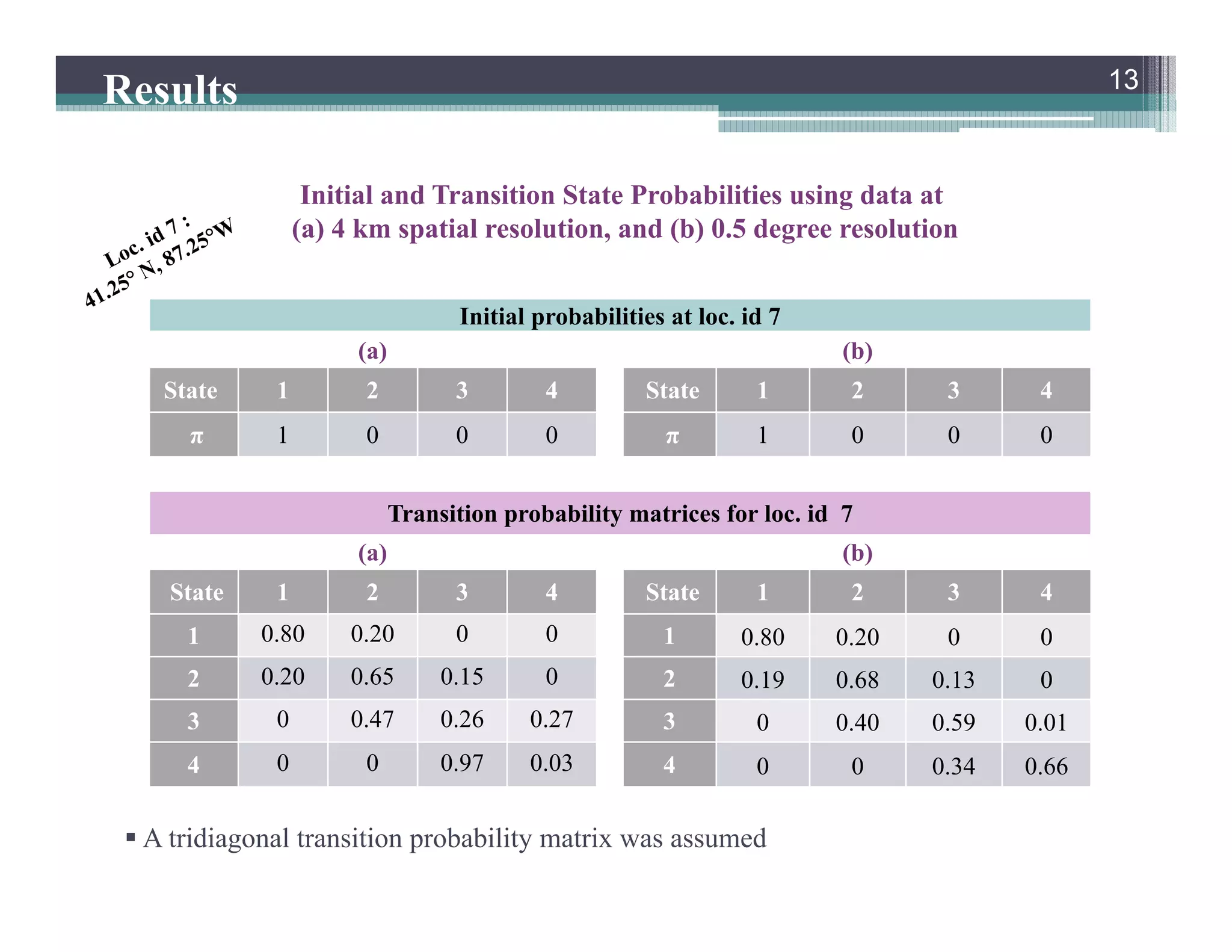
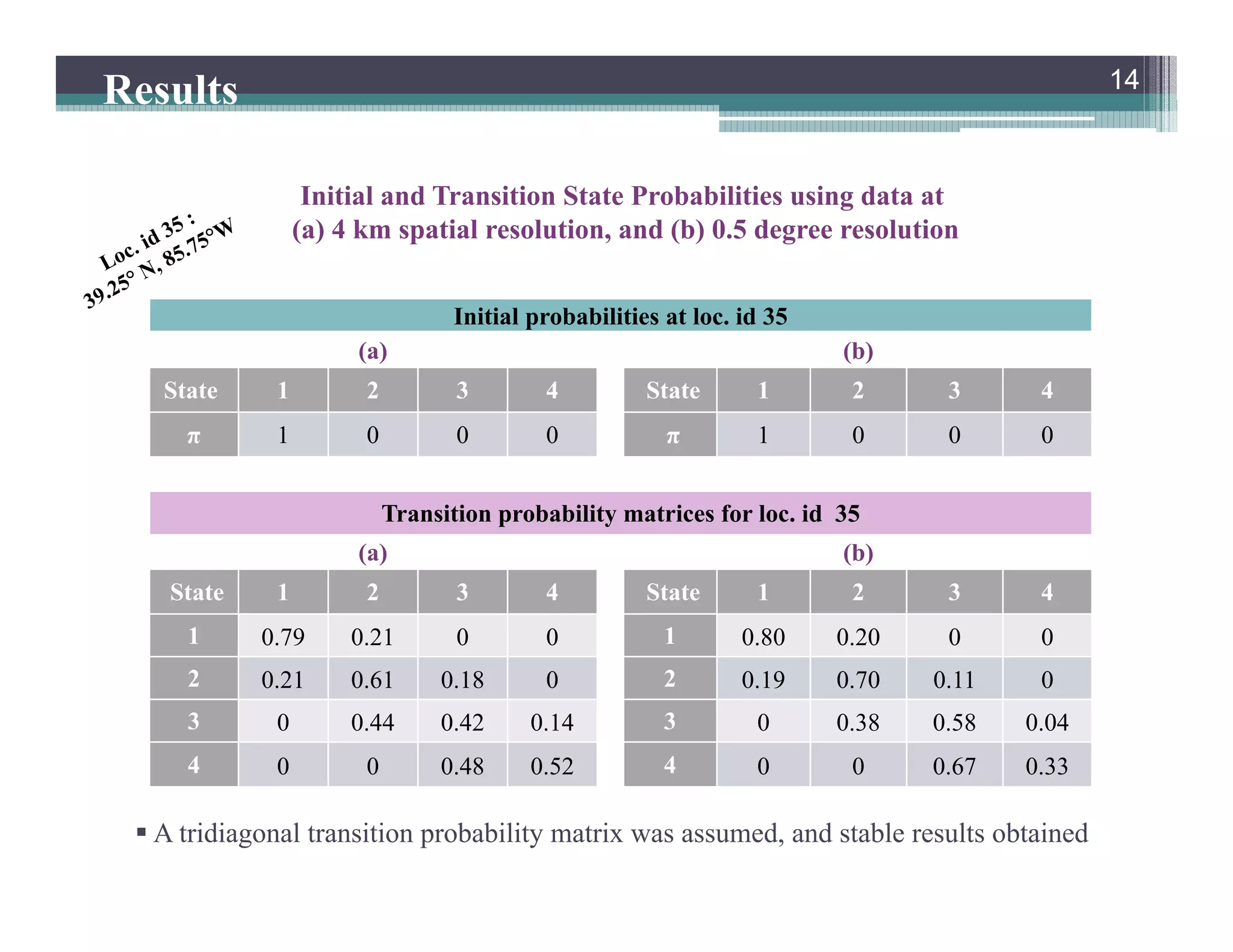
• Parameter estimation consists of determining of the HMM from
the crop water stress time series.
• Continuous Gaussian HMMs are easily modeled. Closed-form expressions
derived for Expectation Maximization (EM) algorithm [Rabiner, 1989].
• Crop stress values are however bounded in the range of [0,1]. Beta
emission distribution was found suitable for the emission model.
Derivation of new parameter estimation formula was performed from first
principles of EM algorithm.
• These expressions are obtained by treating parameter estimation as a
constrained optimization of Probability of Observations given the Model
parameters or P(O|model), subject to constraints, and estimation formula
are developed using Lagrange multipliers technique.
9
{ , , }A B
9](https://image.slidesharecdn.com/probalisticassessmentofagriculture-140807095346-phpapp01/75/Probalistic-assessment-of-agriculture-9-2048.jpg)
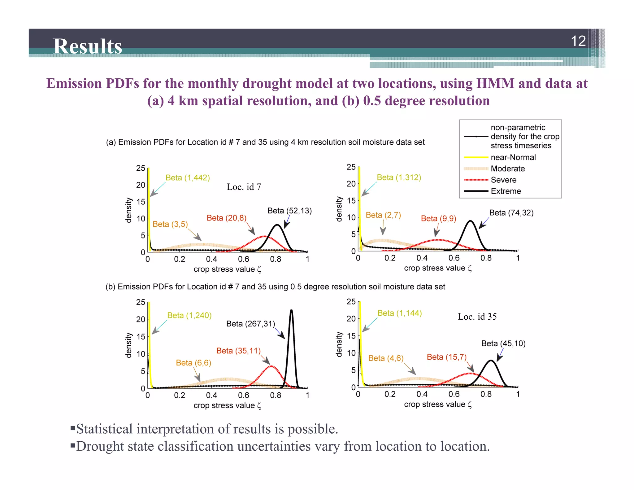
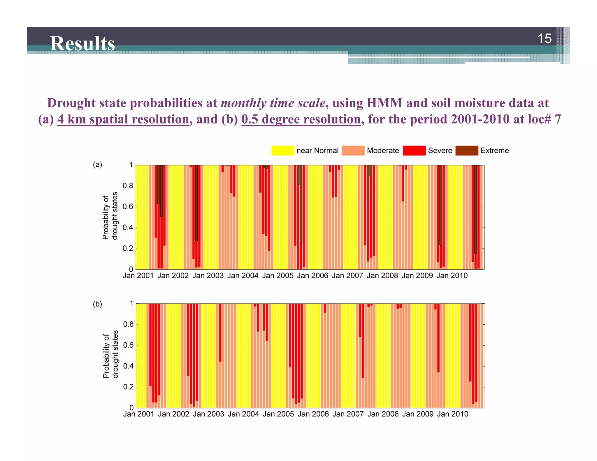
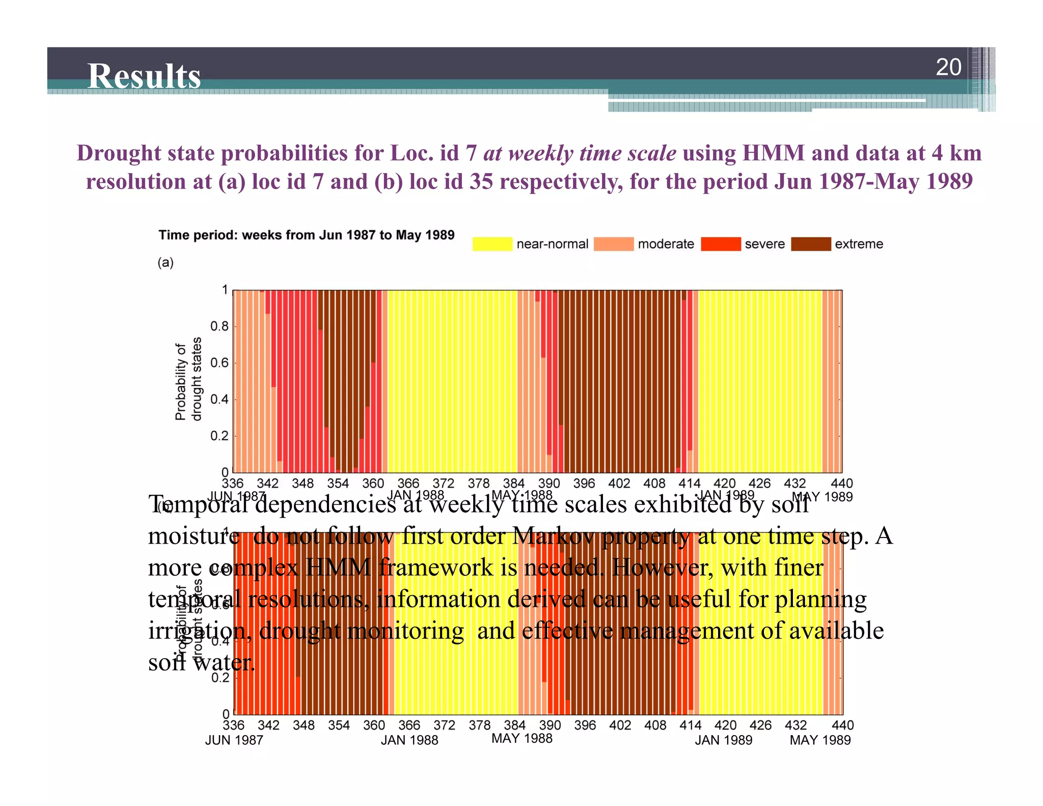

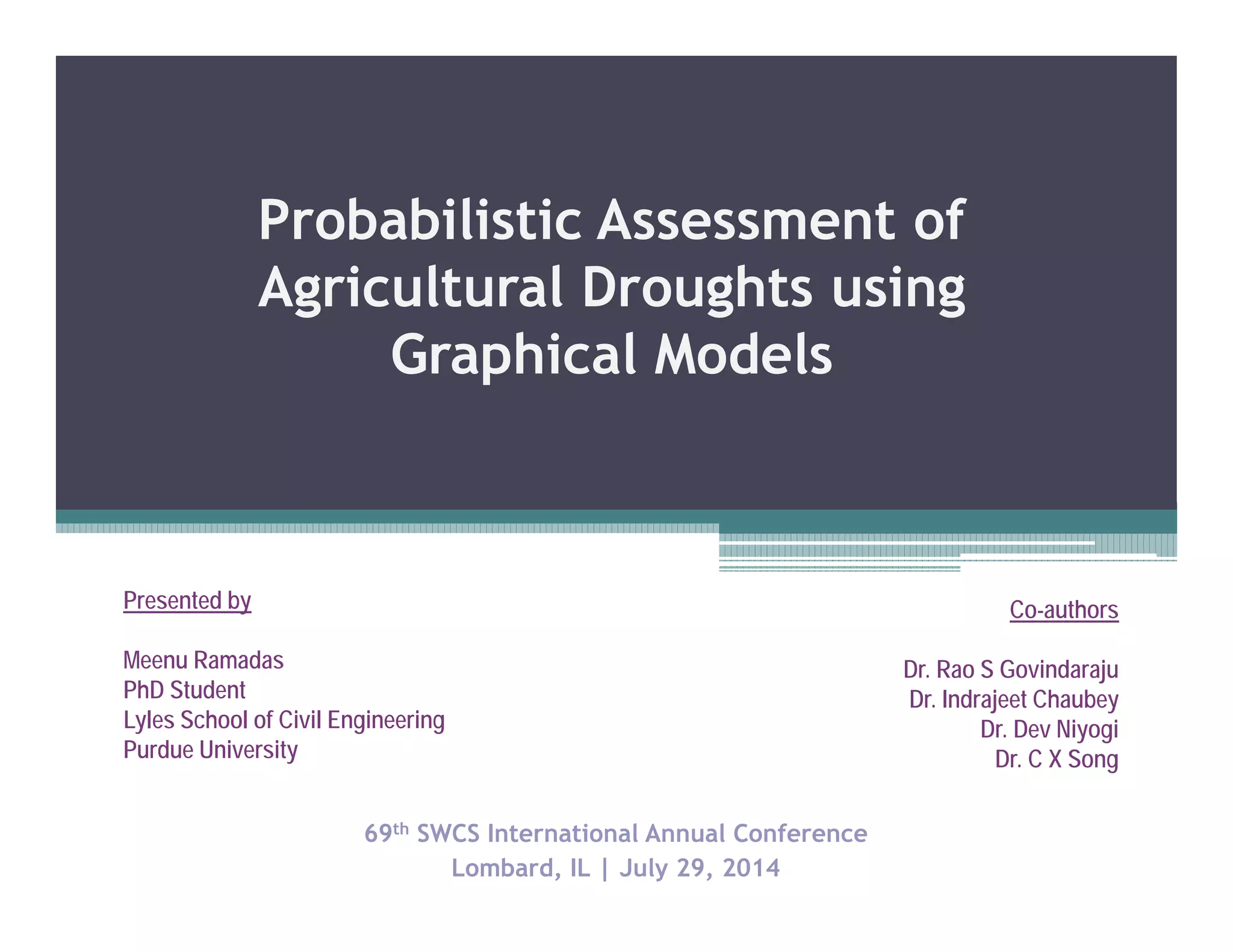
This document summarizes a study that developed a probabilistic model for assessing agricultural droughts using graphical models. The study used hidden Markov models (HMMs) to relate unobserved drought states to observed crop water stress levels. HMMs were estimated using soil moisture and crop data at different spatial scales in Indiana. Results showed drought classifications varied by location and resolution. The probabilistic approach provided uncertainty estimates not available from other drought indices and identified additional drought events. Weekly analyses revealed complex temporal dependencies requiring advanced HMM frameworks.