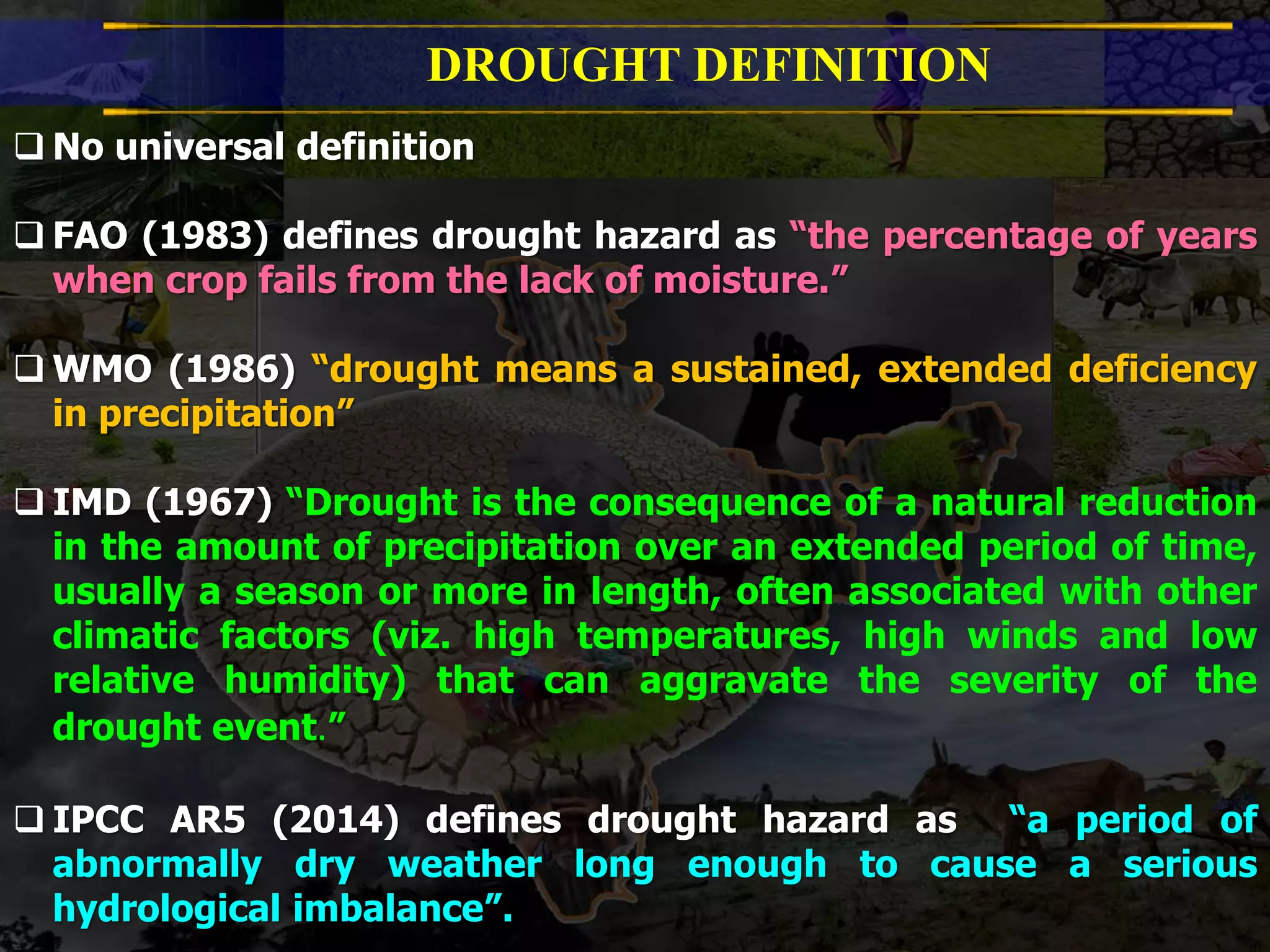
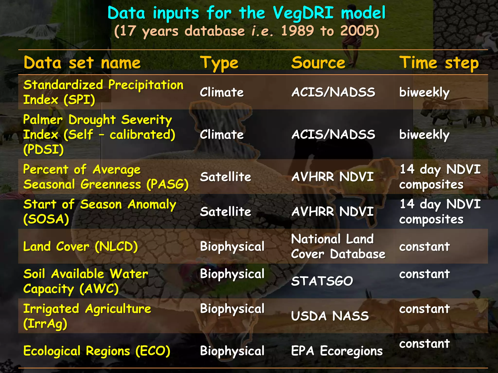
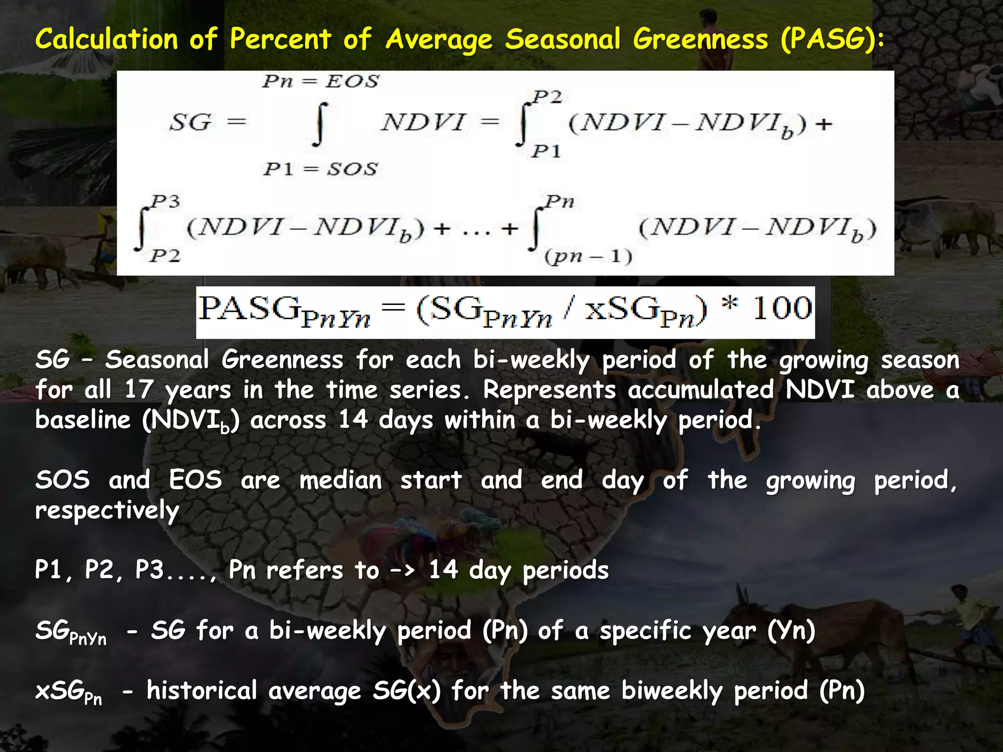
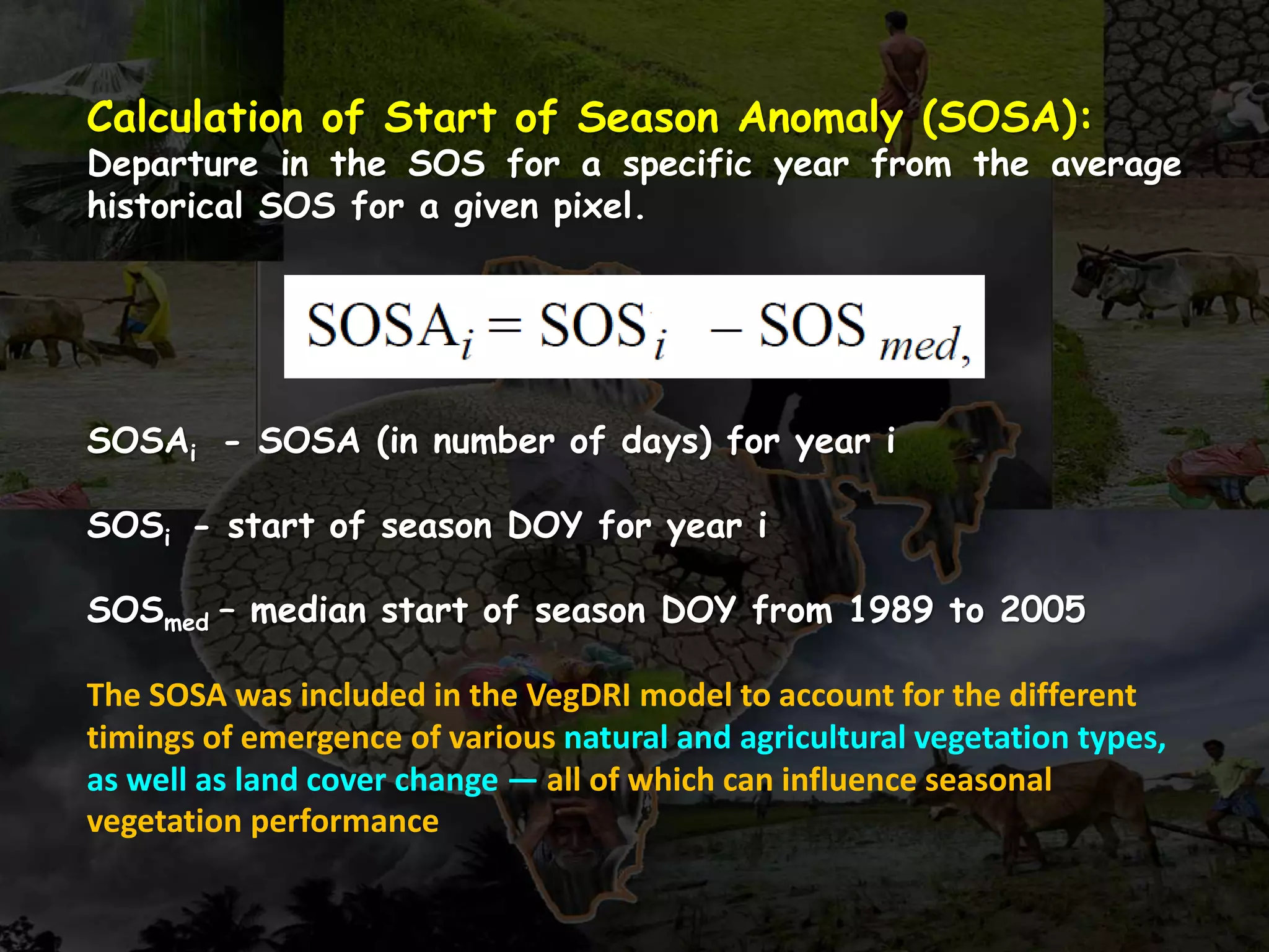
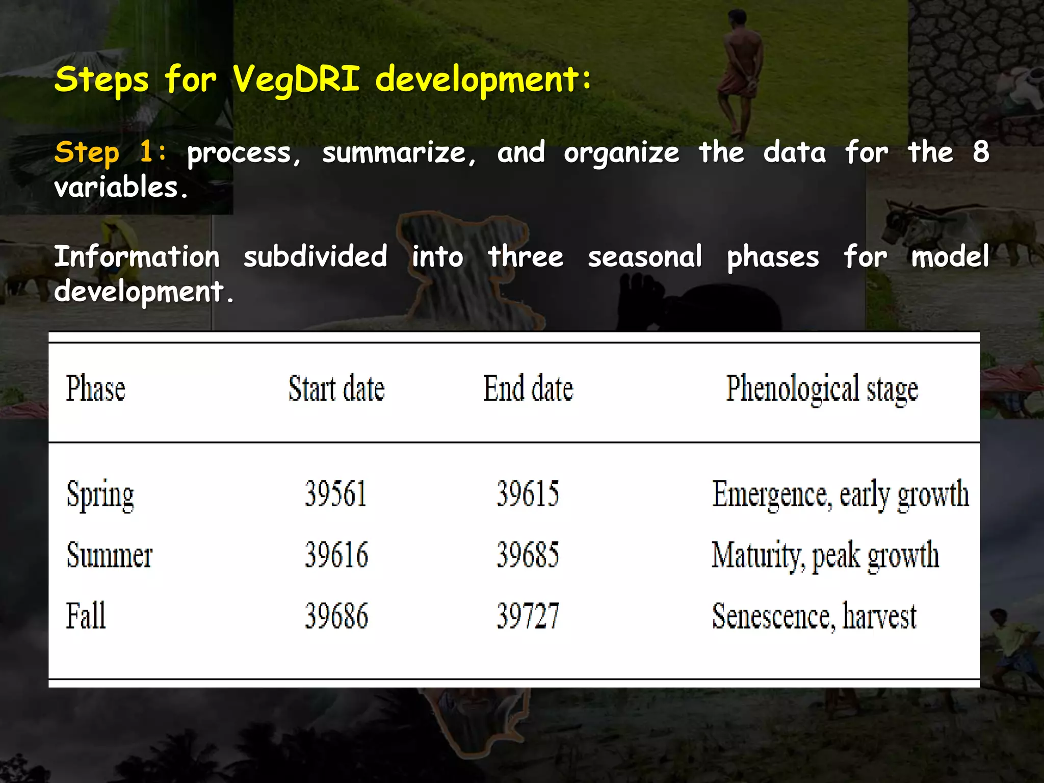
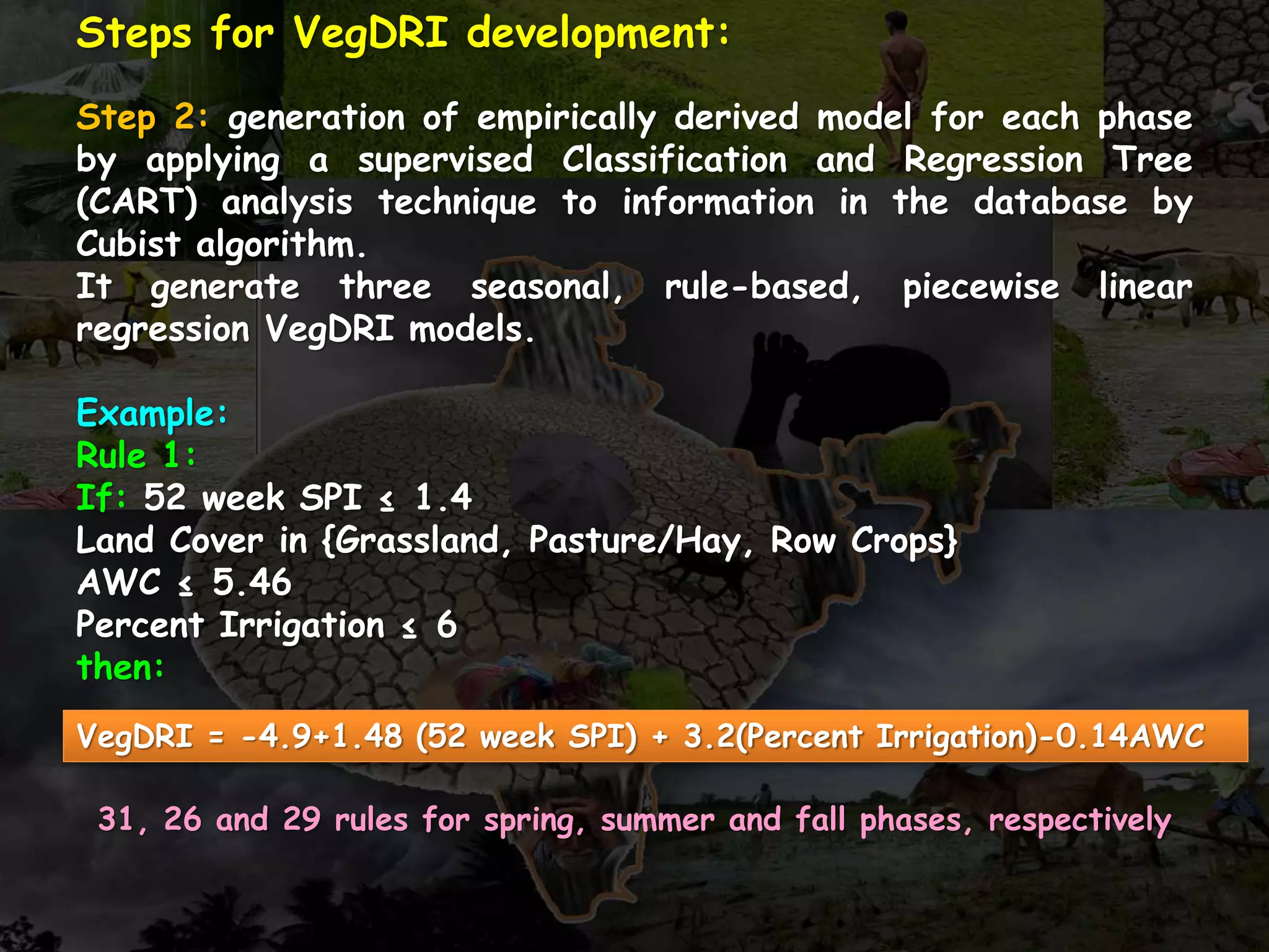
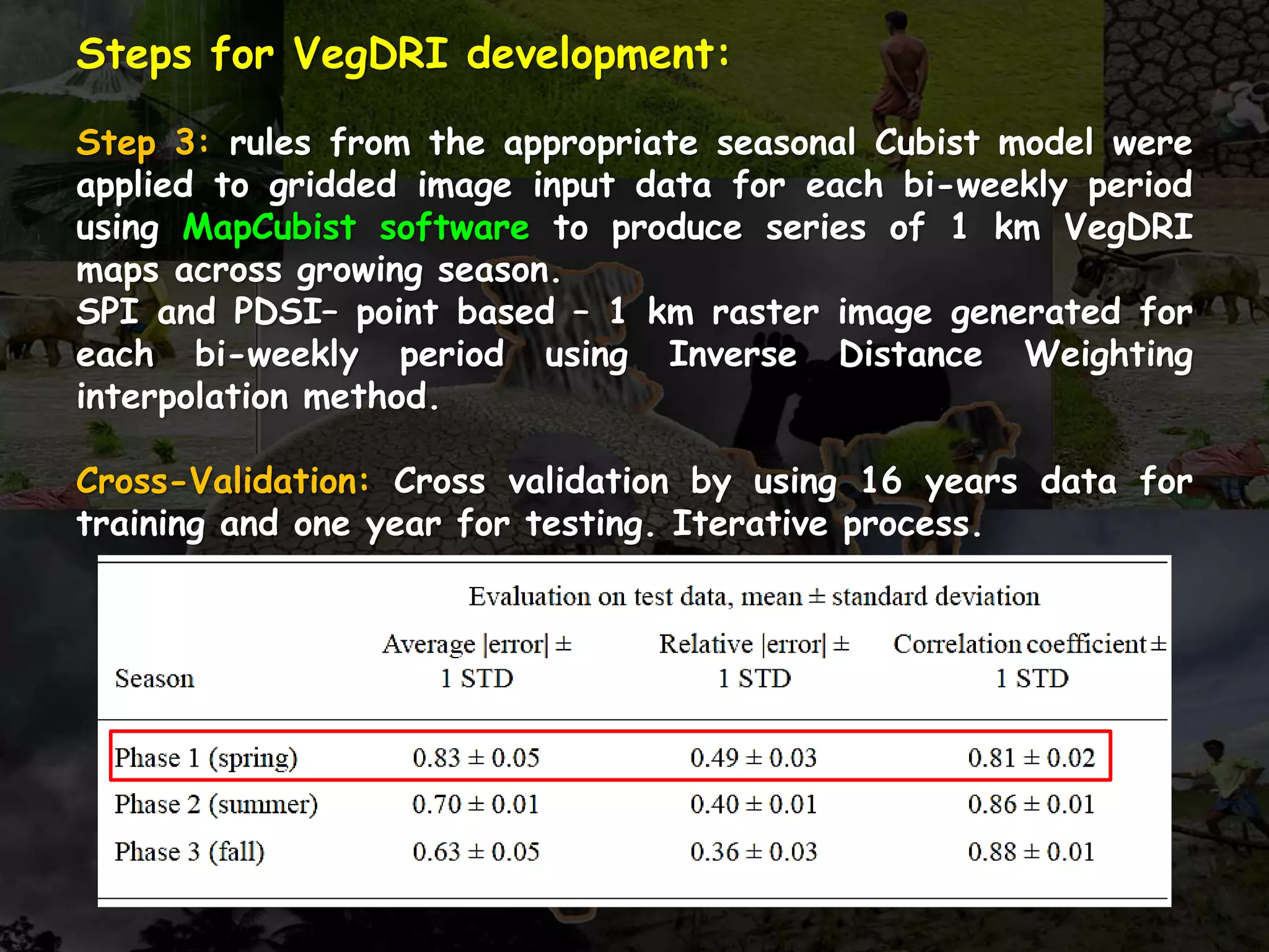
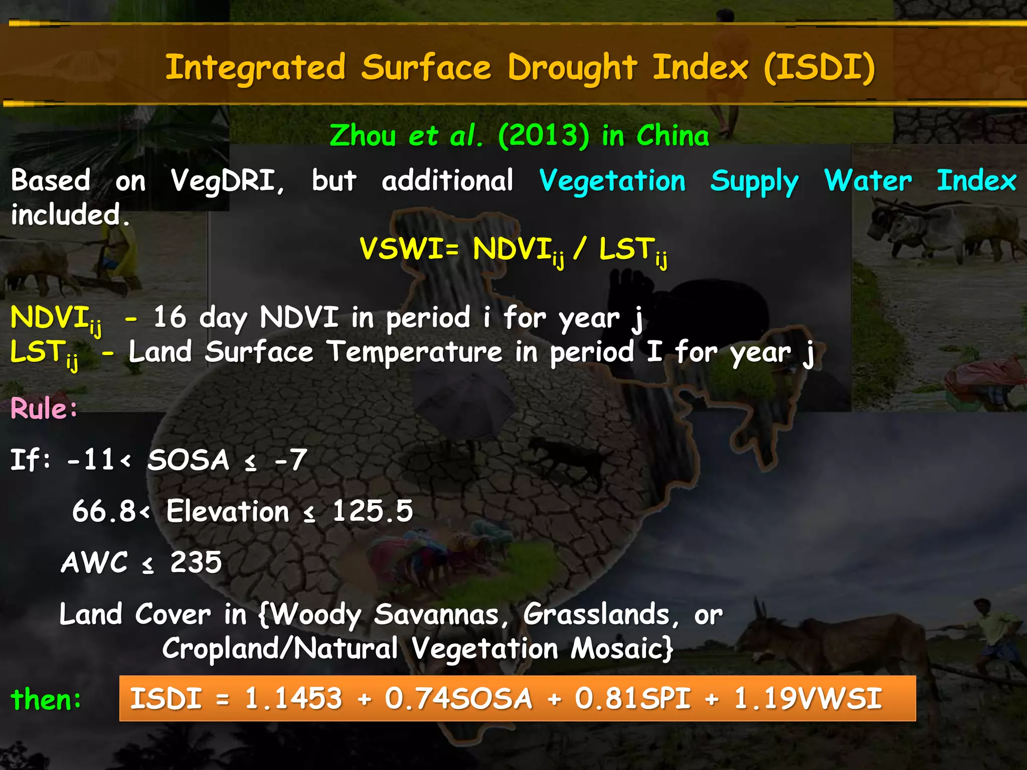
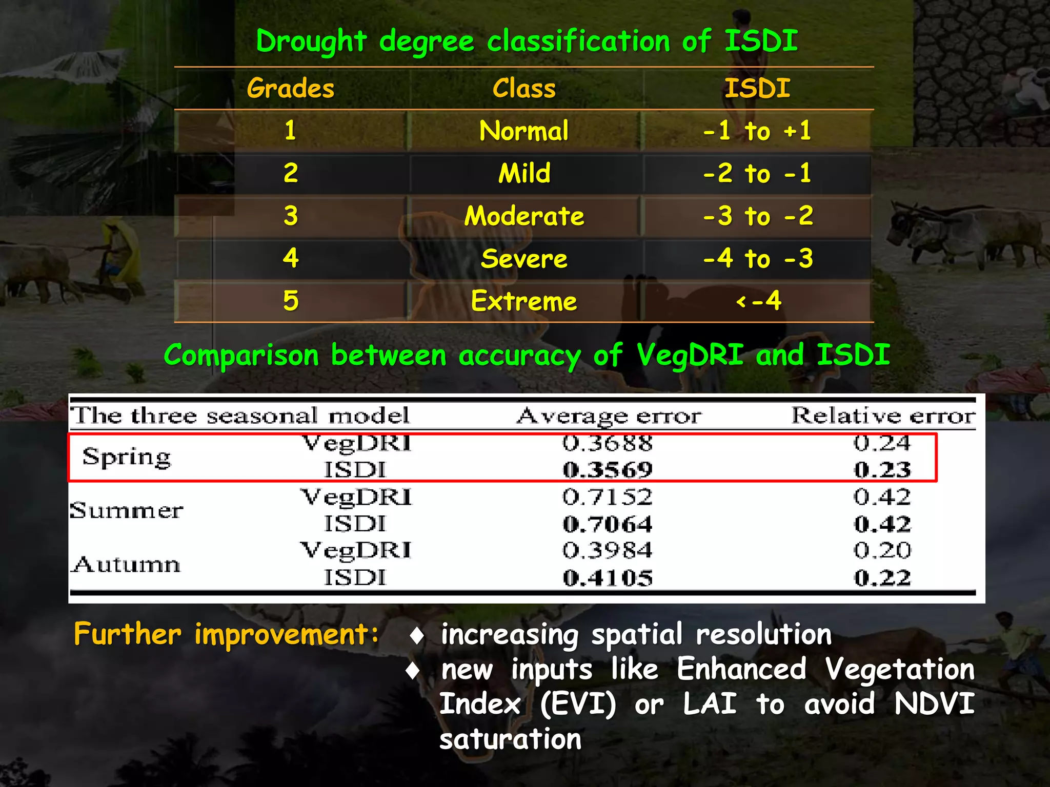
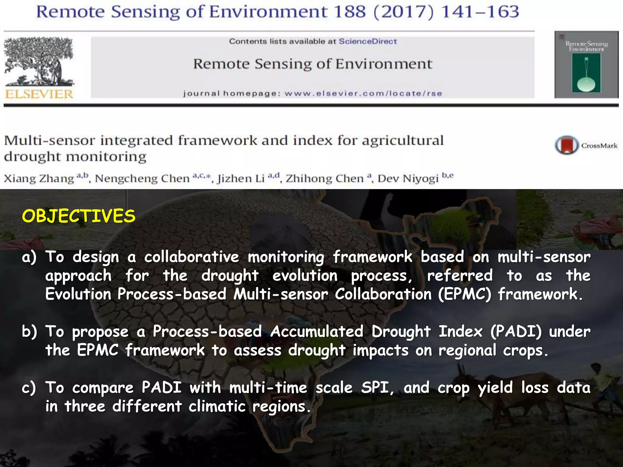
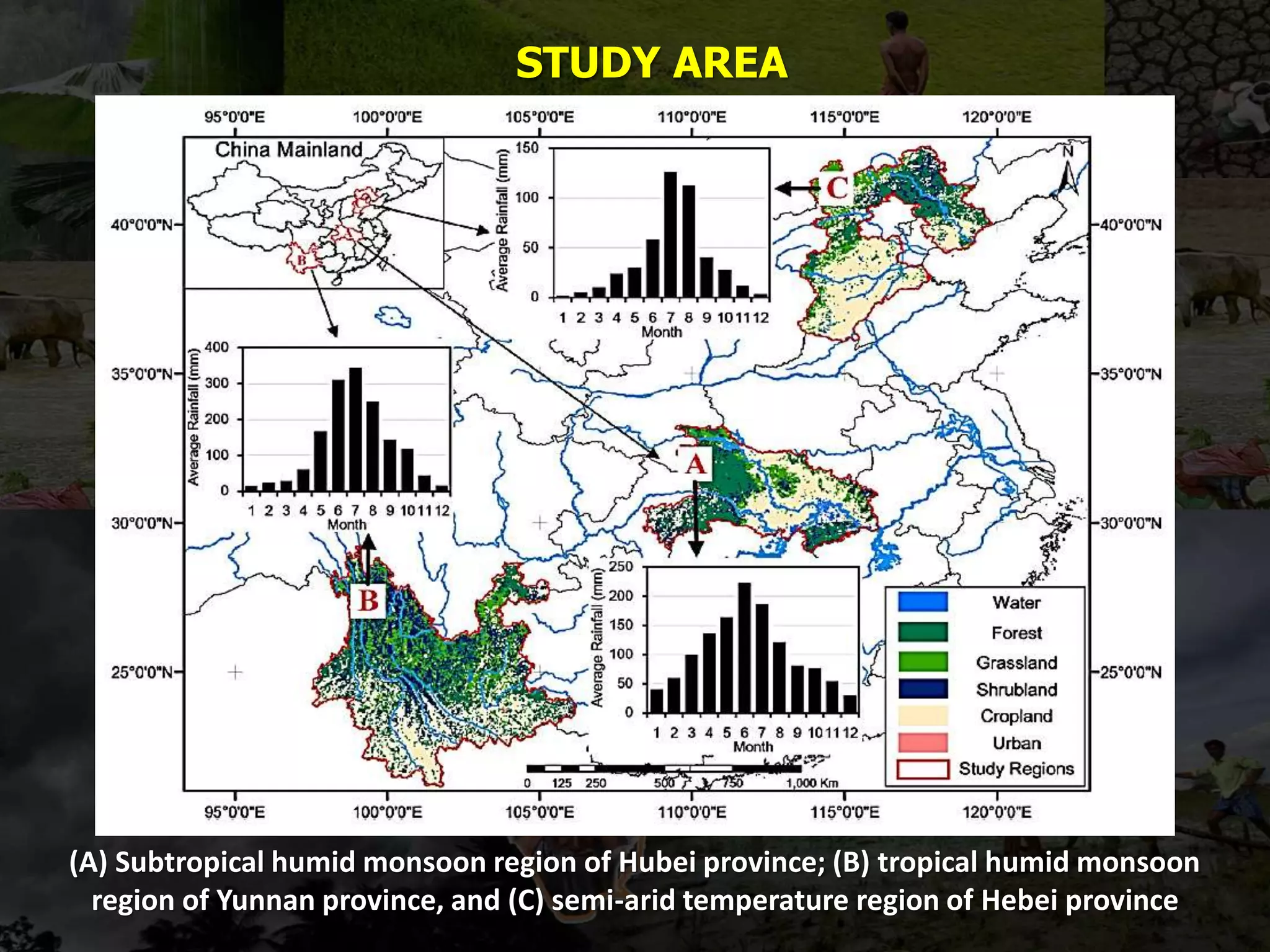
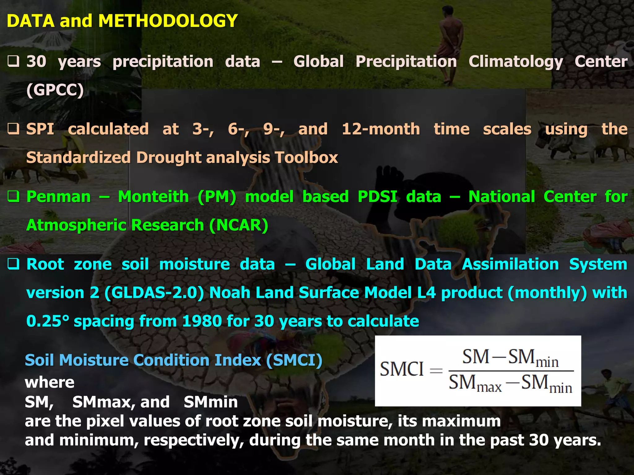
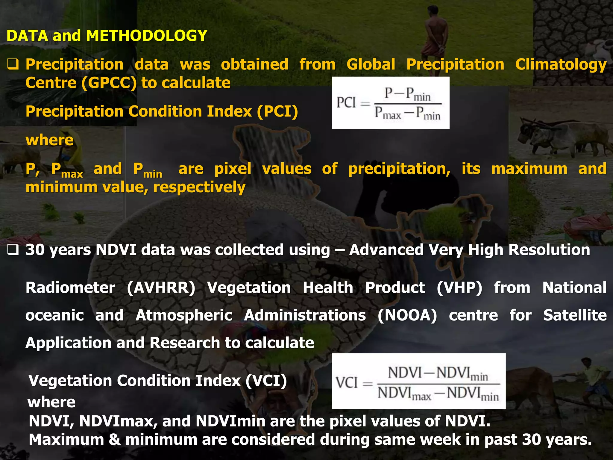
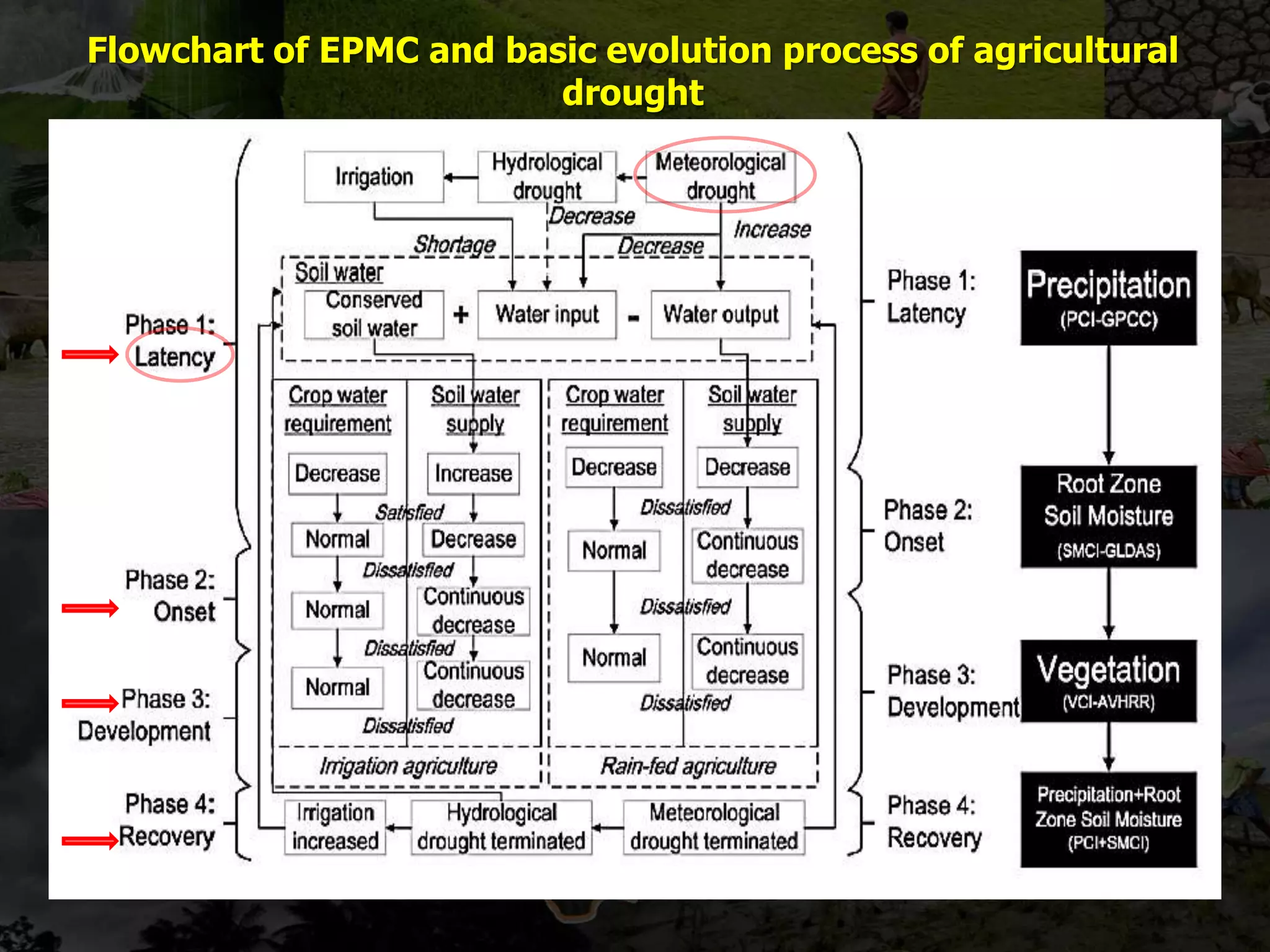
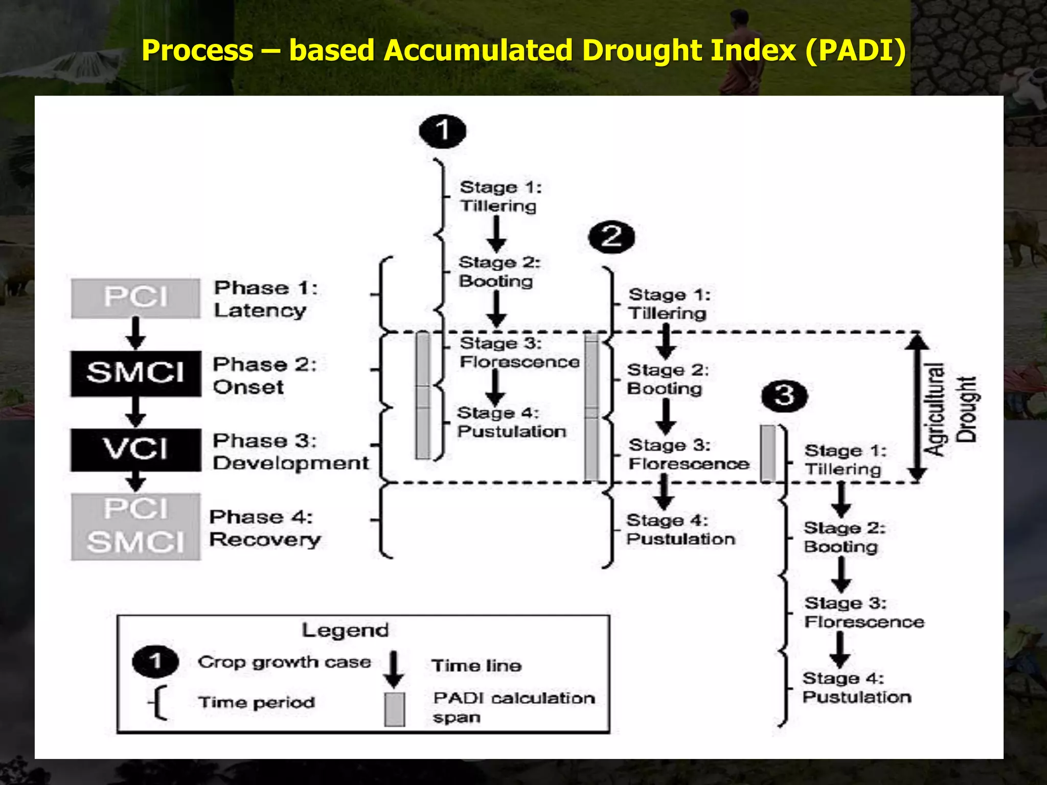
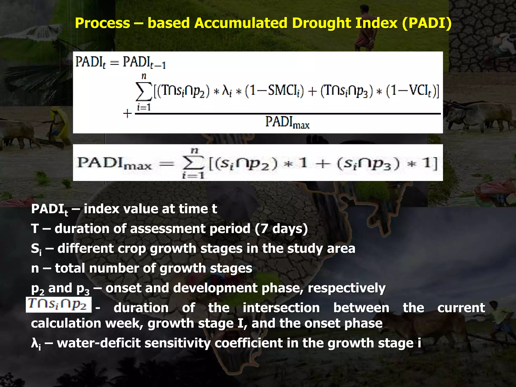
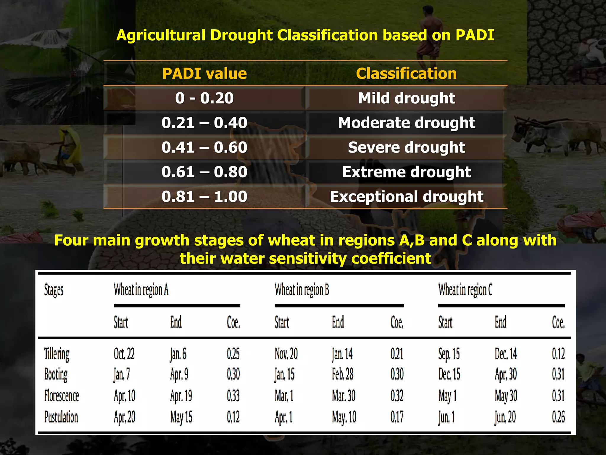
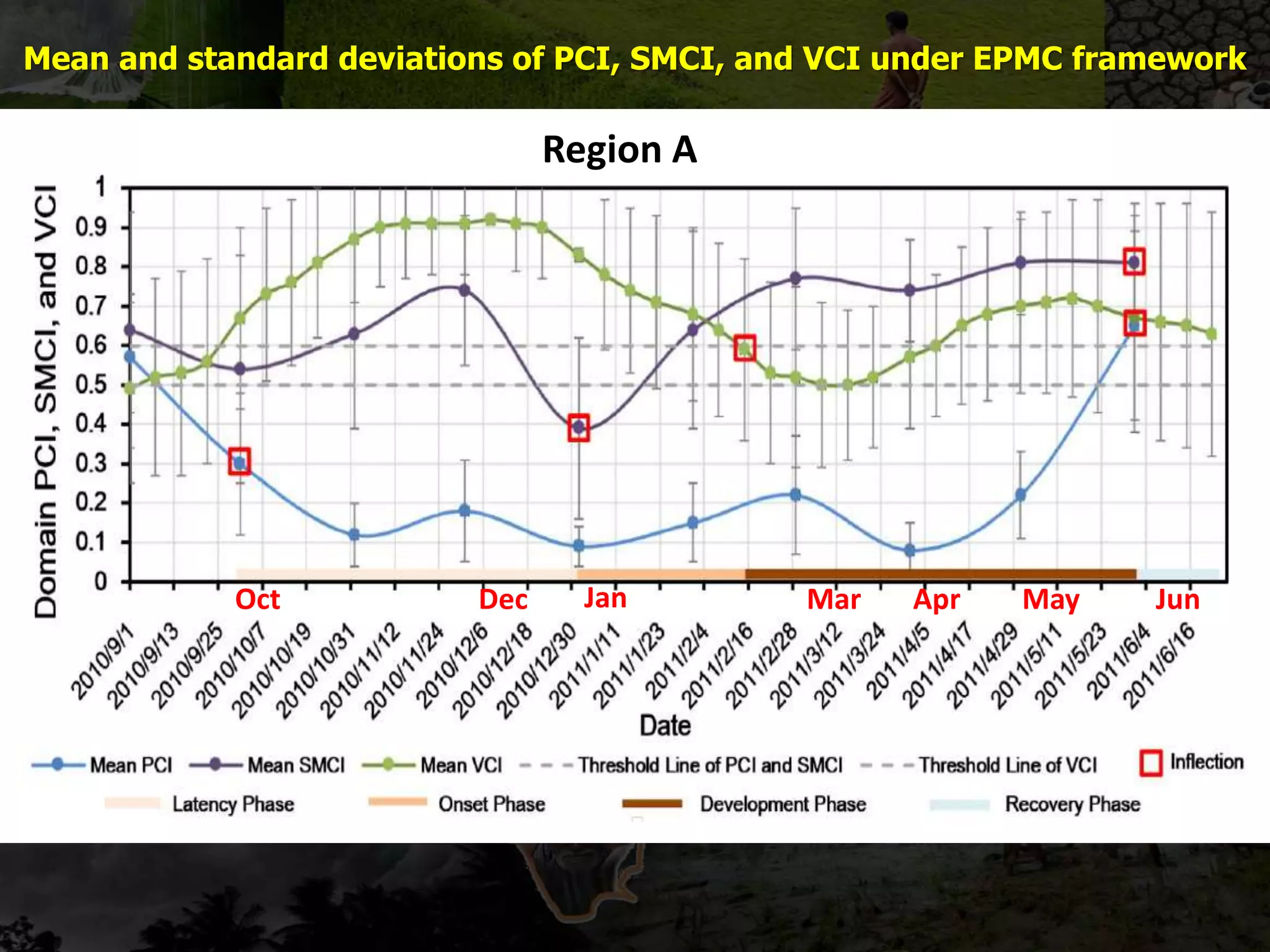
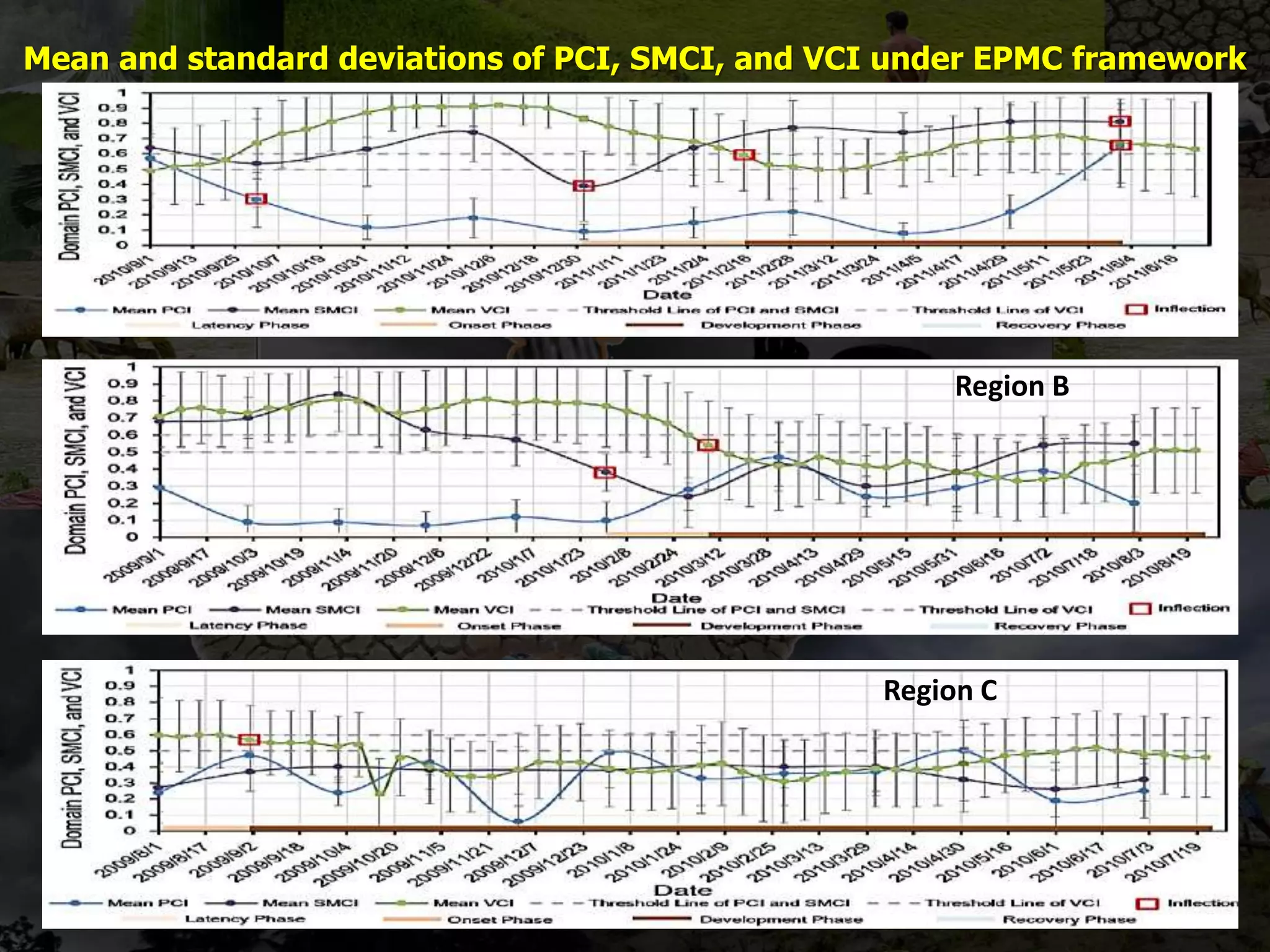
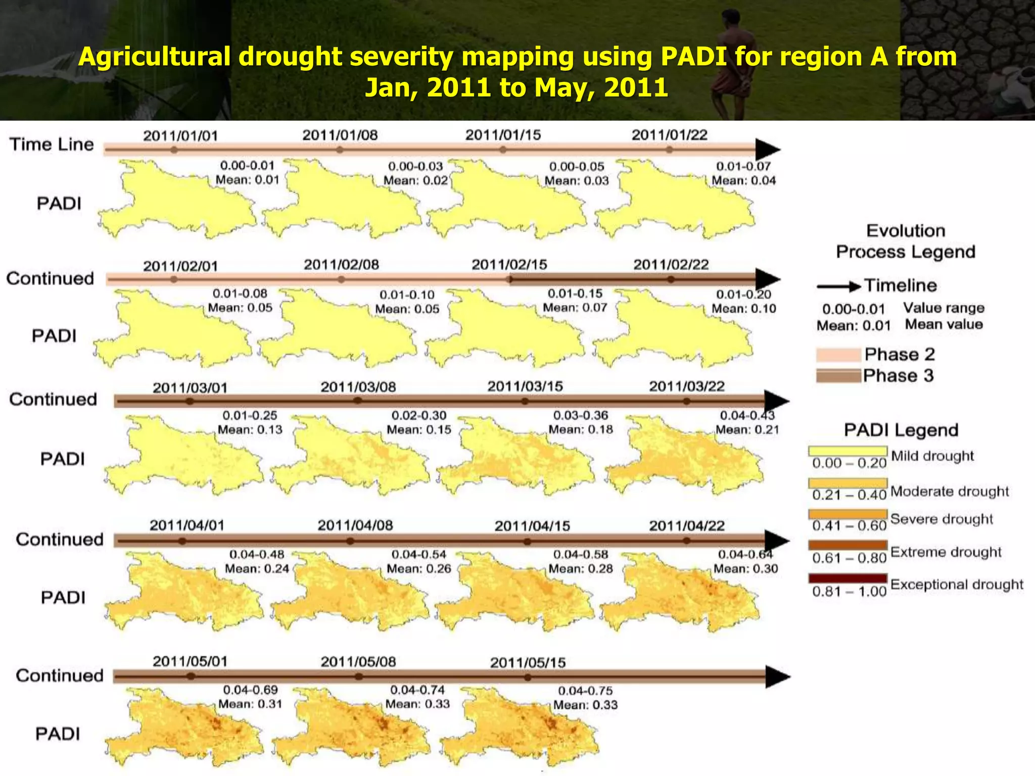
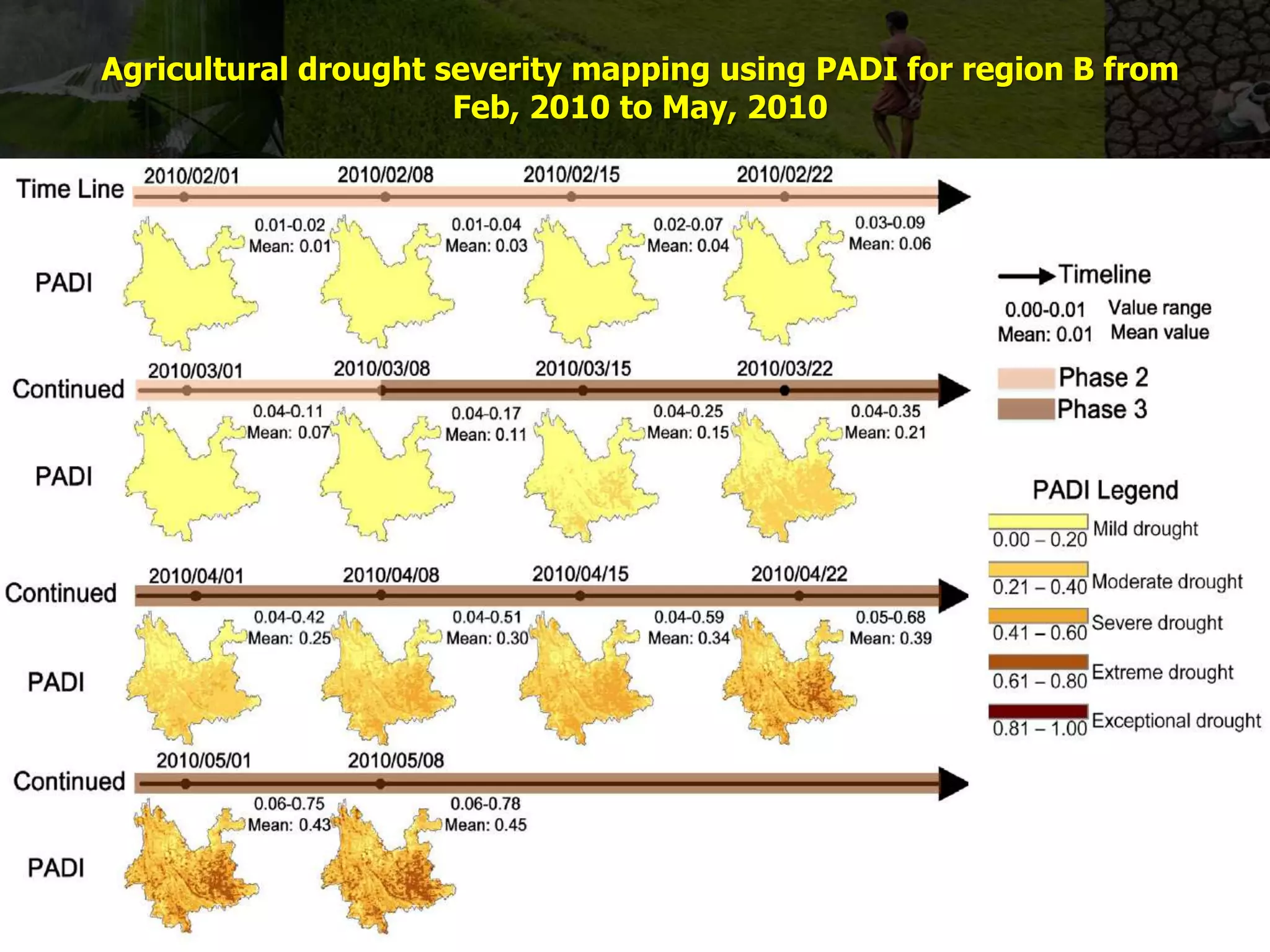
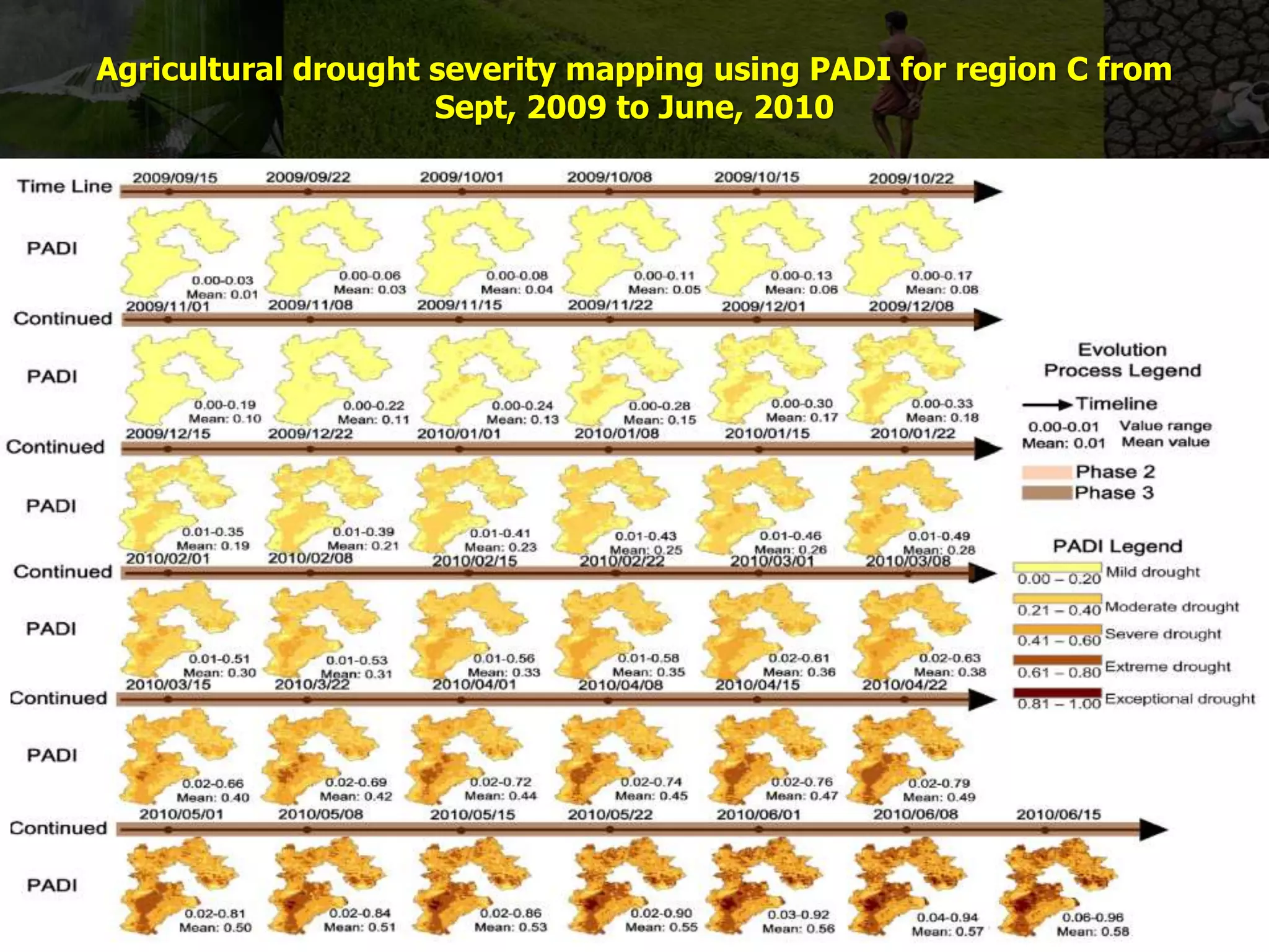
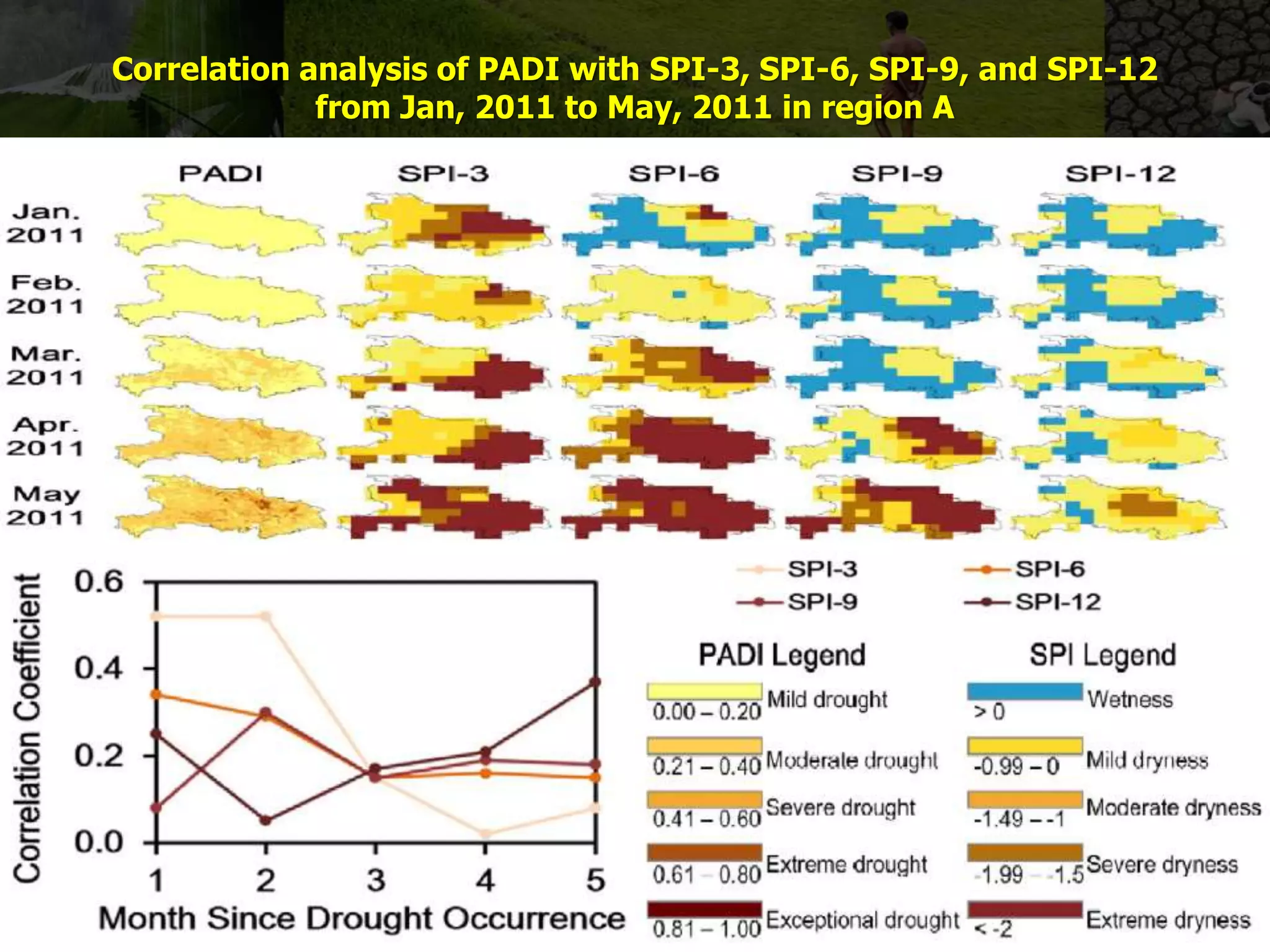
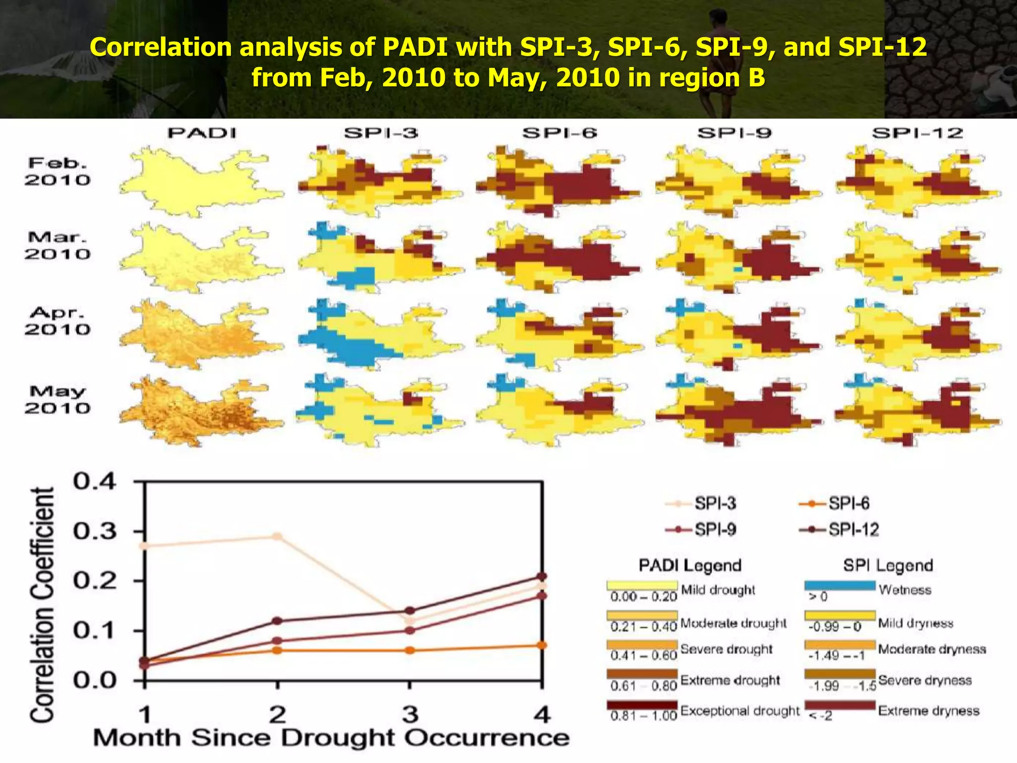
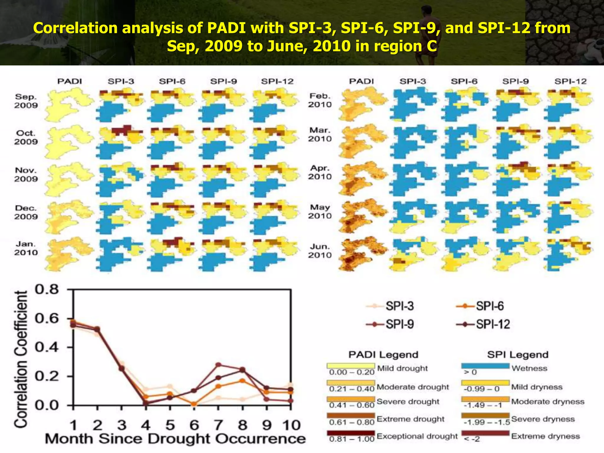
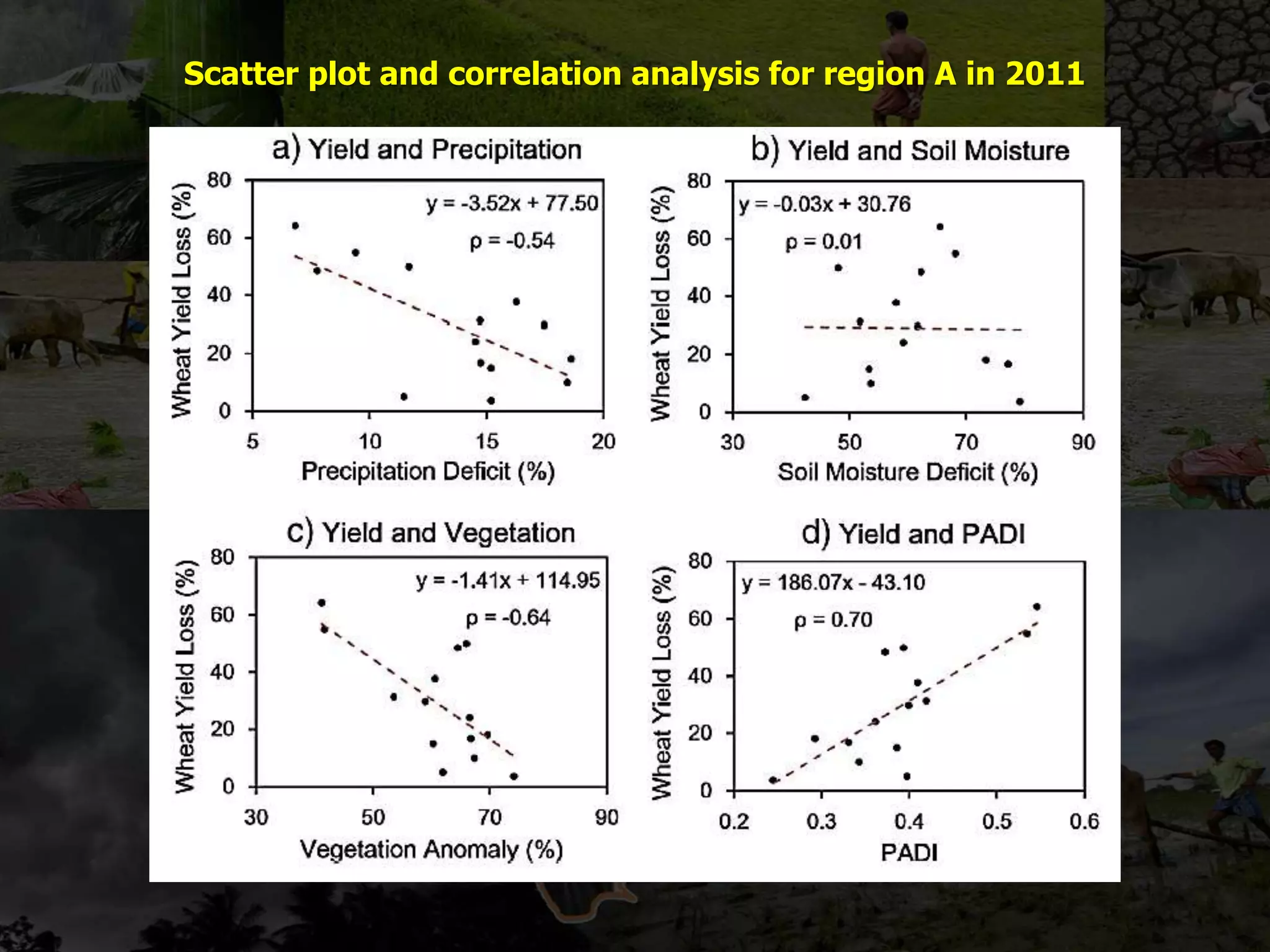
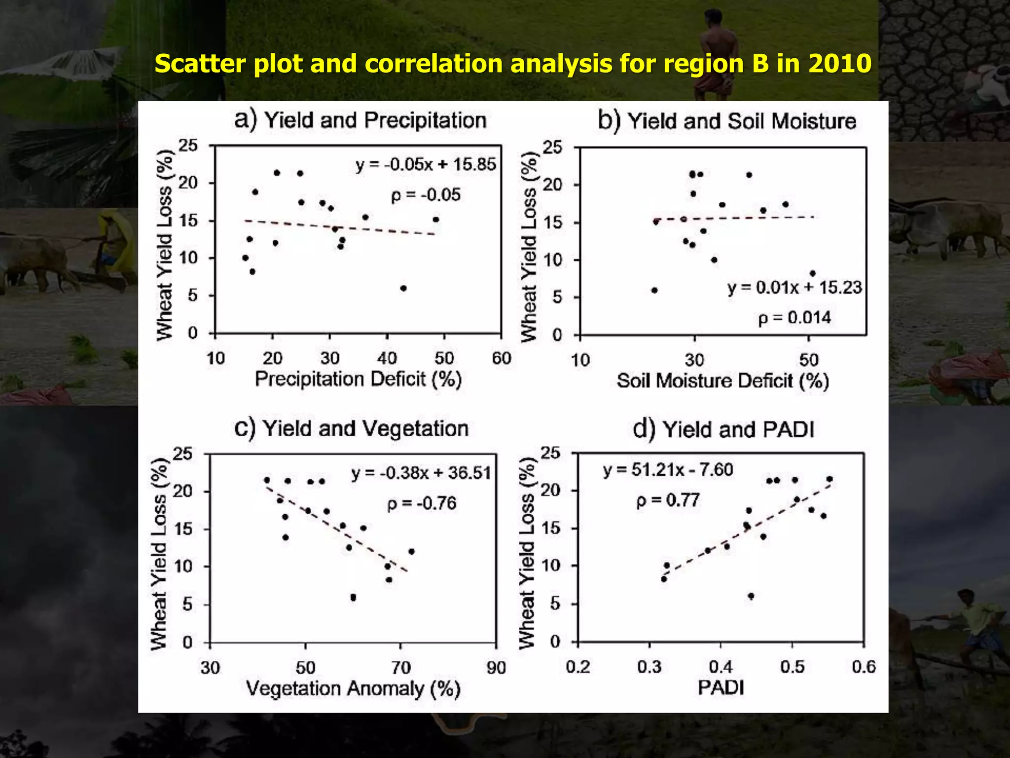
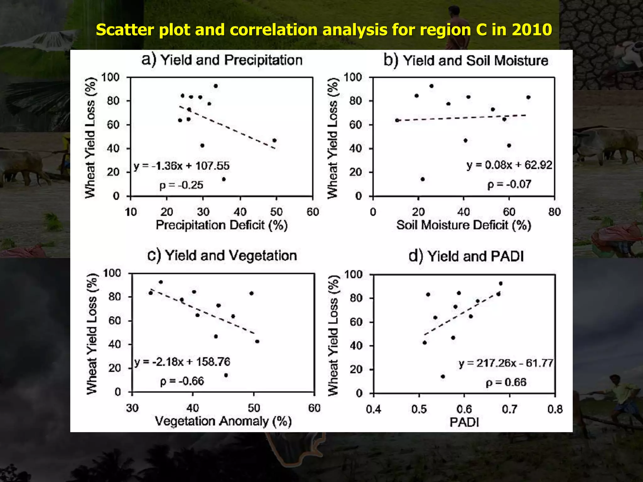
ABHILASH
Ph.D. Student
Dept. of Agricultural Meteorology
CCS Haryana Agricultural University, Hisar
DROUGHT DEFINITION
 No universal definition
 FAO (1983) defines drought hazard as “the percentage of years
when crop fails from the lack of moisture.”
 WMO (1986) “drought means a sustained, extended deficiency
in precipitation”
 IMD (1967) “Drought is the consequence of a natural reduction
in the amount of precipitation over an extended period of time,
usually a season or more in length, often associated with other
climatic factors (viz. high temperatures, high winds and low
relative humidity) that can aggravate the severity of the
drought event.”
 IPCC AR5 (2014) defines drought hazard as “a period of
abnormally dry weather long enough to cause a serious
hydrological imbalance”.
Source: National Drought Mitigation Center, University of Nebraska – Lincoln, U.S.A
Natural Climatic Variability
Precipitation deficiency High temperature, high
winds, low R.H., greater
sunshine, less cloud cover
Soil water deficiency
Plant water stress,
reduced biomass and yield
Reduced stream flow,
inflow to reservoirs, lakes
and ponds
HydrologicalAgriculturalMeteorological
DroughtDroughtDrought
Socio-economic impact
Time(duration)
Importance of Monitoring and Forecasting of
Agricultural Drought
 The frequency of drought in India is increasing.
1950-1990 – 10 drought years
since 2000 – 6 drought years (2002, 2004, 2009, 2014 ,2015 and 2016)
 68 % of the net sown area in India is prone to drought.
 Monitoring and forecasting are part of preparedness that helps in
reducing the impact of drought by following practices:
 Selection of crop management practices
 Contingency planning
 Policy formulation
 Crop/ Livestock insurance
 Watershed management
 Agro-advisories
 Monitoring helps in providing relief measures to severely affected
areas.
AGRICULTURAL DROUGHT INDICES
Indices Author Description Advantages Limitations
Standardized
Precipitation
Index (SPI)
McKee et
al. (1992) at
Colorado
State
University,
USA
Uses only
precipitation
data
Simple and
measures
drought
conditions at
different time
scales
Use only
precipitation, hard
to
interpolate over
large areas
Standardized
Precipitation
Evapotranspiratio
n Index (SPEI)
Vicente-
Serrano
(2010) at
Pyrenean
Institute of
Ecology,
Spain
Based on SPI
requiring
precipitation and
PET data
Simple, adaptable
to different time
scales and
regions, spatial
comparison
possible
Accuracy depends
upon length of
precipitation and
temperature
record
Stress Degree
Days (SDD)
Jackson
et al.,
(1977)
Uses Canopy and
air temperature
A simple measure
calculated by the
difference
between canopy
and air
temperature
Environmental
conditions such as
air
humidity and soil
moisture can
affect
the index
AGRICULTURAL DROUGHT INDICES
Indices Author Description Advantages Limitations
Palmer Drought
Severity Index
(PDSI)
Palmer
(1965)
Uses precipitation
and temperature
to estimate
moisture supply
and demand in soil
Calculate soil
moisture content
to estimate
drought
Slow respone; less
suited for higher
elevation and
winter period
having snow
Crop Moisture
Index (CMI)
Palmer
(1968)
Uses Weekly
precipitation,
weekly mean
temperature and
previous week’s
CMI value.
Identifies
potential
agricultural
droughts
Not useful in long
term drought
monitoring
Crop Specific
Drought Index
(CSDI)
Meyer
et al.
(early
1990s) at
the
University
of
Nebraska-
Lincoln
Uses temperature,
precipitation and
evapotranspiration
data
Provides daily
estimates of soil
water
availability for
different zones
and
soil layers
Too many
requirements
including soil
type, crop
phenology, and
climatological
data
AGRICULTURAL DROUGHT INDICES
Indices Author Description Advantages Limitations
Aridity Anomaly
Index (AAI)
Developed in
India by IMD
Based on
Thornthwaite’s
(1948) water
balance
technique
AET and PET values
are used
Simple calculations.
Responds quickly
with a weekly time
step.
Not applicable
to long-term
or
multiseasonal
events
Soil Moisture
Deficit Index
(SMDI)
Narasimhan
and Srinivasan
(2004) at the
Texas
Agricultural
Experiment
Station, United
States
Weekly soil
moisture and
ET values
simulated by the
Soil and Water
Assessment Tool
(SWAT)
Improves the ability
for modeling
and monitoring
hydrological system &
soil moisture deficit
at a finer
Resolution
Irrespective to
soil properties
across
different
climatic
conditions
Normalized
Difference
Vegetation Index
(NDVI)
Developed by
Tarpley et al.
and Kogan
while working
with NOAA,
United States
(1984)
(NIR-R)/(NIR+R)
Simple Calculations.
Measure crop
vigour
Slow to
respond
Solar Induced Chlorophyll Fluorescence (SIF)
 Extracted by Joiner et al. (2014) using GOME – 2 spectrometer onboard
MetOp – A satellite at 740 nm using radiative transfer model.
 First study for drought monitoring and assessment – Wang et al.
(2016) in the great plains of U.S.A. mainly South Dakota (39),
Nebraska (25) and Kansas (14)
Correlation coefficients of short term SPIs and SIF, NDVI and NDWI from June to August,
2012. Results of Climatic Divisions 1401, 1402, 2501 and 3901 are indicated by (a – d),
respectively. ‘n’ is sample number for regression analysis and ‘p’ is lowest significance
level
For SPI-3 (Lower values are
deeper red which indicate less
precipitation)
%SIF reduction in
2012
%NDVI reduction in
2012
Lack of precipitation over the Great Plains from May to October in 2012
The Vegetation Drought Response Index (VegDRI): A New
Integrated Approach for Monitoring Drought Stress in
Vegetation
(Brown et al. ,2008)
 VegDRI integrates historical climate data and satellite – based earth
observations with other biophysical parameters to produce 1 km resolution
indicator of the geographical extent and intensity of drought stress on
vegetation
 Study conducted over seven state regions of United States for 2002
7 states with
geographic locations of
776 weather stations
used for VegDRI
development
Data inputs for the VegDRI model
(17 years database i.e. 1989 to 2005)
Data set name Type Source Time step
Standardized Precipitation
Index (SPI)
Climate ACIS/NADSS biweekly
Palmer Drought Severity
Index (Self – calibrated)
(PDSI)
Climate ACIS/NADSS biweekly
Percent of Average
Seasonal Greenness (PASG)
Satellite AVHRR NDVI
14 day NDVI
composites
Start of Season Anomaly
(SOSA)
Satellite AVHRR NDVI
14 day NDVI
composites
Land Cover (NLCD) Biophysical
National Land
Cover Database
constant
Soil Available Water
Capacity (AWC)
Biophysical
STATSGO
constant
Irrigated Agriculture
(IrrAg)
Biophysical
USDA NASS
constant
Ecological Regions (ECO) Biophysical EPA Ecoregions
constant
Calculation of Percent of Average Seasonal Greenness (PASG):
SG – Seasonal Greenness for each bi-weekly period of the growing season
for all 17 years in the time series. Represents accumulated NDVI above a
baseline (NDVIb) across 14 days within a bi-weekly period.
SOS and EOS are median start and end day of the growing period,
respectively
P1, P2, P3...., Pn refers to –> 14 day periods
SGPnYn - SG for a bi-weekly period (Pn) of a specific year (Yn)
xSGPn - historical average SG(x) for the same biweekly period (Pn)
Calculation of Start of Season Anomaly (SOSA):
Departure in the SOS for a specific year from the average
historical SOS for a given pixel.
SOSAi - SOSA (in number of days) for year i
SOSi - start of season DOY for year i
SOSmed – median start of season DOY from 1989 to 2005
The SOSA was included in the VegDRI model to account for the different
timings of emergence of various natural and agricultural vegetation types,
as well as land cover change — all of which can influence seasonal
vegetation performance
Steps for VegDRI development:
Step 1: process, summarize, and organize the data for the 8
variables.
Information subdivided into three seasonal phases for model
development.
Steps for VegDRI development:
Step 2: generation of empirically derived model for each phase
by applying a supervised Classification and Regression Tree
(CART) analysis technique to information in the database by
Cubist algorithm.
It generate three seasonal, rule-based, piecewise linear
regression VegDRI models.
Example:
Rule 1:
If: 52 week SPI ≤ 1.4
Land Cover in {Grassland, Pasture/Hay, Row Crops}
AWC ≤ 5.46
Percent Irrigation ≤ 6
then:
VegDRI = -4.9+1.48 (52 week SPI) + 3.2(Percent Irrigation)-0.14AWC
31, 26 and 29 rules for spring, summer and fall phases, respectively
Steps for VegDRI development:
Step 3: rules from the appropriate seasonal Cubist model were
applied to gridded image input data for each bi-weekly period
using MapCubist software to produce series of 1 km VegDRI
maps across growing season.
SPI and PDSI– point based – 1 km raster image generated for
each bi-weekly period using Inverse Distance Weighting
interpolation method.
Cross-Validation: Cross validation by using 16 years data for
training and one year for testing. Iterative process.
Results
VegDRI map for March
10, 2015
USDM map for March
12, 2015
Integrated Surface Drought Index (ISDI)
Zhou et al. (2013) in China
Based on VegDRI, but additional Vegetation Supply Water Index
included.
VSWI= NDVIij / LSTij
NDVIij - 16 day NDVI in period i for year j
LSTij - Land Surface Temperature in period I for year j
Rule:
If: -11< SOSA ≤ -7
66.8< Elevation ≤ 125.5
AWC ≤ 235
Land Cover in {Woody Savannas, Grasslands, or
Cropland/Natural Vegetation Mosaic}
then: ISDI = 1.1453 + 0.74SOSA + 0.81SPI + 1.19VWSI
Further improvement:  increasing spatial resolution
 new inputs like Enhanced Vegetation
Index (EVI) or LAI to avoid NDVI
saturation
Drought degree classification of ISDI
Grades Class ISDI
1 Normal -1 to +1
2 Mild -2 to -1
3 Moderate -3 to -2
4 Severe -4 to -3
5 Extreme <-4
Comparison between accuracy of VegDRI and ISDI
OBJECTIVES
a) To design a collaborative monitoring framework based on multi-sensor
approach for the drought evolution process, referred to as the
Evolution Process-based Multi-sensor Collaboration (EPMC) framework.
b) To propose a Process-based Accumulated Drought Index (PADI) under
the EPMC framework to assess drought impacts on regional crops.
c) To compare PADI with multi-time scale SPI, and crop yield loss data
in three different climatic regions.
STUDY AREA
(A) Subtropical humid monsoon region of Hubei province; (B) tropical humid monsoon
region of Yunnan province, and (C) semi-arid temperature region of Hebei province
DATA and METHODOLOGY
 30 years precipitation data – Global Precipitation Climatology Center
(GPCC)
 SPI calculated at 3-, 6-, 9-, and 12-month time scales using the
Standardized Drought analysis Toolbox
 Penman – Monteith (PM) model based PDSI data – National Center for
Atmospheric Research (NCAR)
 Root zone soil moisture data – Global Land Data Assimilation System
version 2 (GLDAS-2.0) Noah Land Surface Model L4 product (monthly) with
0.25° spacing from 1980 for 30 years to calculate
Soil Moisture Condition Index (SMCI)
where
SM, SMmax, and SMmin
are the pixel values of root zone soil moisture, its maximum
and minimum, respectively, during the same month in the past 30 years.
DATA and METHODOLOGY
 Precipitation data was obtained from Global Precipitation Climatology
Centre (GPCC) to calculate
Precipitation Condition Index (PCI)
where
P, Pmax and Pmin are pixel values of precipitation, its maximum and
minimum value, respectively
 30 years NDVI data was collected using – Advanced Very High Resolution
Radiometer (AVHRR) Vegetation Health Product (VHP) from National
oceanic and Atmospheric Administrations (NOOA) centre for Satellite
Application and Research to calculate
Vegetation Condition Index (VCI)
where
NDVI, NDVImax, and NDVImin are the pixel values of NDVI.
Maximum & minimum are considered during same week in past 30 years.
Flowchart of EPMC and basic evolution process of agricultural
drought
Process – based Accumulated Drought Index (PADI)
PADIt – index value at time t
T – duration of assessment period (7 days)
Si – different crop growth stages in the study area
n – total number of growth stages
p2 and p3 – onset and development phase, respectively
- duration of the intersection between the current
calculation week, growth stage I, and the onset phase
λi – water-deficit sensitivity coefficient in the growth stage i
Agricultural Drought Classification based on PADI
PADI value Classification
0 - 0.20 Mild drought
0.21 – 0.40 Moderate drought
0.41 – 0.60 Severe drought
0.61 – 0.80 Extreme drought
0.81 – 1.00 Exceptional drought
Four main growth stages of wheat in regions A,B and C along with
their water sensitivity coefficient
Mean and standard deviations of PCI, SMCI, and VCI under EPMC framework
Region A
Oct Dec Jan Mar Apr May Jun
Mean and standard deviations of PCI, SMCI, and VCI under EPMC framework
Region B
Region C
Agricultural drought severity mapping using PADI for region A from
Jan, 2011 to May, 2011
Agricultural drought severity mapping using PADI for region B from
Feb, 2010 to May, 2010
Agricultural drought severity mapping using PADI for region C from
Sept, 2009 to June, 2010
Correlation analysis of PADI with SPI-3, SPI-6, SPI-9, and SPI-12
from Jan, 2011 to May, 2011 in region A
Correlation analysis of PADI with SPI-3, SPI-6, SPI-9, and SPI-12
from Feb, 2010 to May, 2010 in region B
Correlation analysis of PADI with SPI-3, SPI-6, SPI-9, and SPI-12 from
Sep, 2009 to June, 2010 in region C
Scatter plot and correlation analysis for region A in 2011
Scatter plot and correlation analysis for region B in 2010
Scatter plot and correlation analysis for region C in 2010
Predicting agricultural drought in eastern Rajasthan of
India using NDVI and standardized precipitation index
Dutta et al. (2013)
Study area
STUDY AREA 
METHODOLOGY
 Rainfall data : Daily data from 1984 to 2003 was used for
SPI computation
 Crop yield statistics : three major kharif crops i.e. sorghum,
pearl millet and maize of each 21 districts of Eastern
Rajasthan from http://www.rajasthankrishi.gov.in
 Satellite data : NDVI derived from AVHRR onboard NOAA. 15
day composite with spatial resolution of 8 km.
 Multiple Regression Model with two variables, SPI and
previous NDVI, used to predict NDVI of coming fortnight
 Regression model was developed for predicting dominant
crop yield from NDVI
RESULTS
Correlation coefficients at different agro-climatic zones
NDVI prediction models
Multiple Regression Models for NDVI prediction in the transitional
zone
Note: SPI-1 = SPI of previous fortnight, NDVI-1 = NDVI of previous fortnight,
SPI 3 = cumulative rainfall of previous three fortnights, SPI 6 = cumulative rainfall of
previous 6 fortnights and SEE = standard error of estimate
NDVI prediction models
Multiple Regression Models for NDVI prediction in the semi-arid zone
Note: SPI-1 = SPI of previous fortnight, NDVI-1 = NDVI of previous fortnight,
SPI 3 = cumulative rainfall of previous three fortnights, SPI 6 = cumulative rainfall of
previous 6 fortnights and SEE = standard error of estimate
Predicted and observed NDVI in (A) drought year 2002, and
(B) non-drought year 2003
Transitional Zone
Semi-arid Zone
Correlation coefficients of fortnightly NDVI and sorghum yield
Crop yield prediction models
Observed and predicted yield of dominant crop
OBJECTIVES
a) Develop a drought forecast model based on the combination of
remote sensing and long-range forecast data using machine
learning for ungauged areas
b) Provide improved ranges of drought forecast in case of the
improvement of forecasting skill of the long-range forecast data
Study area : South Korea
Data:
 Monthly precipitation and temperature data from 61 Automatic Synoptic
Observation System (ASOS)
 Potential Evapotranspiration – mean air temperature using Thornthwaite
method
 SPI and Standardized Precipitation Evapotranspiration Index (SPEI) with
3-, 6-, 9-, and 12- month time scale were used with lead times from 1 to 6
months.
Remote Sensing data used for ungauged stations
Classification Index Value
Extremely Wet (EW) ≥2.00
Very Wet (VW) 1.50 - 1.99
Moderately Wet (MW) 1.00 – 1.49
Near Normal (NN) From 0.99 to – 0.99
Moderate Draught (MD) From -1.00 to -1.49
Severe Drought (SD) From -1.50 to -1.99
Extreme Drought (ED) ≤ -2.00
Drought condition classifications for SPI and SPEI (McKee et al., 1993).
Six Global Climate Models (GCMs) used in this study to obtain long range
climate forecast data
Drought category classification accuracy measures
Drought forecasting at gauge locations
 For each station locations, SPI and SPEI were calculated.
 For each lead time, observation data were used for the past period,
and two methods were used to fill the future period:
1. Climatology data were obtained from the median value of 100
samples randomly derived from the observation data of the same
month (C – method)
2. Long-range forecast data : percent increment of modeled
precipitation or temperature anomaly is applied to observational
climatology data to form the calibrated model data (F – method)
Drought forecasting for ungauged areas
 Following machine learning models (ML – method)
1. Decision Trees (DT)
2. Random forest (RF)
3. Extremely randomized trees (ERT)
 Kriging (gaussian process) as spatial interpolation baseline method
(I – method)
Structure of each machine learning model
RESULTS
Producer’s Drought Accuracy of SPI and SPEI forecasts with 3-, 6-, 9-, and 12-month
time scales and lead times of 1–6 months based on C-method and F-method.
Producer’s Drought Accuracy of SPI and SPEI forecasts with 3-, 6-, 9-, and 12-month time
scales and lead times of 1–6 months based on C-I, F-I, C-ML (DT, RF, ERT model), and F-ML
(DT, RF, ERT model) methods
Producer’s Drought Accuracy of SPI and SPEI forecasts with 3-, 6-, 9-, and 12-month time
scales and lead times of 1–6 months based on C-I, F-I, C-ML (DT, RF, ERT model), and F-ML
(DT, RF, ERT model) methods
CONCLUSION
 Drought monitoring accuracy and detail can be improved by
integrating various climate (precipitation and temperature),
vegetation (phenological stage of crop growth) and biophysical (soil
moisture holding capacity, land use change, irrigation and ecological
regions) parameters to produce one drought index through
classification and regression tree approach.
 Considering the cumulative effect of evolution of drought stages on
the respective crop growth stage can further improve the process of
drought monitoring.
 Both fast response factor like SIF and slow response factor like NDVI
is necessary for drought monitoring and forecasting.
 Drought forecasting can be done either by multiple linear regression
model which is region specific and empirical or by new approaches
applicable to every region like Machine Learning which should be
based on large-scale climate indices and long range local
climatological data.
Advances in agricultural drought monitoring and forecasting

Advances in agricultural drought monitoring and forecasting

  • 1.
    ABHILASH Ph.D. Student Dept. ofAgricultural Meteorology CCS Haryana Agricultural University, Hisar
  • 2.
    DROUGHT DEFINITION  Nouniversal definition  FAO (1983) defines drought hazard as “the percentage of years when crop fails from the lack of moisture.”  WMO (1986) “drought means a sustained, extended deficiency in precipitation”  IMD (1967) “Drought is the consequence of a natural reduction in the amount of precipitation over an extended period of time, usually a season or more in length, often associated with other climatic factors (viz. high temperatures, high winds and low relative humidity) that can aggravate the severity of the drought event.”  IPCC AR5 (2014) defines drought hazard as “a period of abnormally dry weather long enough to cause a serious hydrological imbalance”.
  • 3.
    Source: National DroughtMitigation Center, University of Nebraska – Lincoln, U.S.A Natural Climatic Variability Precipitation deficiency High temperature, high winds, low R.H., greater sunshine, less cloud cover Soil water deficiency Plant water stress, reduced biomass and yield Reduced stream flow, inflow to reservoirs, lakes and ponds HydrologicalAgriculturalMeteorological DroughtDroughtDrought Socio-economic impact Time(duration)
  • 4.
    Importance of Monitoringand Forecasting of Agricultural Drought  The frequency of drought in India is increasing. 1950-1990 – 10 drought years since 2000 – 6 drought years (2002, 2004, 2009, 2014 ,2015 and 2016)  68 % of the net sown area in India is prone to drought.  Monitoring and forecasting are part of preparedness that helps in reducing the impact of drought by following practices:  Selection of crop management practices  Contingency planning  Policy formulation  Crop/ Livestock insurance  Watershed management  Agro-advisories  Monitoring helps in providing relief measures to severely affected areas.
  • 5.
    AGRICULTURAL DROUGHT INDICES IndicesAuthor Description Advantages Limitations Standardized Precipitation Index (SPI) McKee et al. (1992) at Colorado State University, USA Uses only precipitation data Simple and measures drought conditions at different time scales Use only precipitation, hard to interpolate over large areas Standardized Precipitation Evapotranspiratio n Index (SPEI) Vicente- Serrano (2010) at Pyrenean Institute of Ecology, Spain Based on SPI requiring precipitation and PET data Simple, adaptable to different time scales and regions, spatial comparison possible Accuracy depends upon length of precipitation and temperature record Stress Degree Days (SDD) Jackson et al., (1977) Uses Canopy and air temperature A simple measure calculated by the difference between canopy and air temperature Environmental conditions such as air humidity and soil moisture can affect the index
  • 6.
    AGRICULTURAL DROUGHT INDICES IndicesAuthor Description Advantages Limitations Palmer Drought Severity Index (PDSI) Palmer (1965) Uses precipitation and temperature to estimate moisture supply and demand in soil Calculate soil moisture content to estimate drought Slow respone; less suited for higher elevation and winter period having snow Crop Moisture Index (CMI) Palmer (1968) Uses Weekly precipitation, weekly mean temperature and previous week’s CMI value. Identifies potential agricultural droughts Not useful in long term drought monitoring Crop Specific Drought Index (CSDI) Meyer et al. (early 1990s) at the University of Nebraska- Lincoln Uses temperature, precipitation and evapotranspiration data Provides daily estimates of soil water availability for different zones and soil layers Too many requirements including soil type, crop phenology, and climatological data
  • 7.
    AGRICULTURAL DROUGHT INDICES IndicesAuthor Description Advantages Limitations Aridity Anomaly Index (AAI) Developed in India by IMD Based on Thornthwaite’s (1948) water balance technique AET and PET values are used Simple calculations. Responds quickly with a weekly time step. Not applicable to long-term or multiseasonal events Soil Moisture Deficit Index (SMDI) Narasimhan and Srinivasan (2004) at the Texas Agricultural Experiment Station, United States Weekly soil moisture and ET values simulated by the Soil and Water Assessment Tool (SWAT) Improves the ability for modeling and monitoring hydrological system & soil moisture deficit at a finer Resolution Irrespective to soil properties across different climatic conditions Normalized Difference Vegetation Index (NDVI) Developed by Tarpley et al. and Kogan while working with NOAA, United States (1984) (NIR-R)/(NIR+R) Simple Calculations. Measure crop vigour Slow to respond
  • 8.
    Solar Induced ChlorophyllFluorescence (SIF)  Extracted by Joiner et al. (2014) using GOME – 2 spectrometer onboard MetOp – A satellite at 740 nm using radiative transfer model.  First study for drought monitoring and assessment – Wang et al. (2016) in the great plains of U.S.A. mainly South Dakota (39), Nebraska (25) and Kansas (14)
  • 9.
    Correlation coefficients ofshort term SPIs and SIF, NDVI and NDWI from June to August, 2012. Results of Climatic Divisions 1401, 1402, 2501 and 3901 are indicated by (a – d), respectively. ‘n’ is sample number for regression analysis and ‘p’ is lowest significance level
  • 10.
    For SPI-3 (Lowervalues are deeper red which indicate less precipitation) %SIF reduction in 2012 %NDVI reduction in 2012 Lack of precipitation over the Great Plains from May to October in 2012
  • 11.
    The Vegetation DroughtResponse Index (VegDRI): A New Integrated Approach for Monitoring Drought Stress in Vegetation (Brown et al. ,2008)  VegDRI integrates historical climate data and satellite – based earth observations with other biophysical parameters to produce 1 km resolution indicator of the geographical extent and intensity of drought stress on vegetation  Study conducted over seven state regions of United States for 2002 7 states with geographic locations of 776 weather stations used for VegDRI development
  • 12.
    Data inputs forthe VegDRI model (17 years database i.e. 1989 to 2005) Data set name Type Source Time step Standardized Precipitation Index (SPI) Climate ACIS/NADSS biweekly Palmer Drought Severity Index (Self – calibrated) (PDSI) Climate ACIS/NADSS biweekly Percent of Average Seasonal Greenness (PASG) Satellite AVHRR NDVI 14 day NDVI composites Start of Season Anomaly (SOSA) Satellite AVHRR NDVI 14 day NDVI composites Land Cover (NLCD) Biophysical National Land Cover Database constant Soil Available Water Capacity (AWC) Biophysical STATSGO constant Irrigated Agriculture (IrrAg) Biophysical USDA NASS constant Ecological Regions (ECO) Biophysical EPA Ecoregions constant
  • 13.
    Calculation of Percentof Average Seasonal Greenness (PASG): SG – Seasonal Greenness for each bi-weekly period of the growing season for all 17 years in the time series. Represents accumulated NDVI above a baseline (NDVIb) across 14 days within a bi-weekly period. SOS and EOS are median start and end day of the growing period, respectively P1, P2, P3...., Pn refers to –> 14 day periods SGPnYn - SG for a bi-weekly period (Pn) of a specific year (Yn) xSGPn - historical average SG(x) for the same biweekly period (Pn)
  • 14.
    Calculation of Startof Season Anomaly (SOSA): Departure in the SOS for a specific year from the average historical SOS for a given pixel. SOSAi - SOSA (in number of days) for year i SOSi - start of season DOY for year i SOSmed – median start of season DOY from 1989 to 2005 The SOSA was included in the VegDRI model to account for the different timings of emergence of various natural and agricultural vegetation types, as well as land cover change — all of which can influence seasonal vegetation performance
  • 15.
    Steps for VegDRIdevelopment: Step 1: process, summarize, and organize the data for the 8 variables. Information subdivided into three seasonal phases for model development.
  • 16.
    Steps for VegDRIdevelopment: Step 2: generation of empirically derived model for each phase by applying a supervised Classification and Regression Tree (CART) analysis technique to information in the database by Cubist algorithm. It generate three seasonal, rule-based, piecewise linear regression VegDRI models. Example: Rule 1: If: 52 week SPI ≤ 1.4 Land Cover in {Grassland, Pasture/Hay, Row Crops} AWC ≤ 5.46 Percent Irrigation ≤ 6 then: VegDRI = -4.9+1.48 (52 week SPI) + 3.2(Percent Irrigation)-0.14AWC 31, 26 and 29 rules for spring, summer and fall phases, respectively
  • 17.
    Steps for VegDRIdevelopment: Step 3: rules from the appropriate seasonal Cubist model were applied to gridded image input data for each bi-weekly period using MapCubist software to produce series of 1 km VegDRI maps across growing season. SPI and PDSI– point based – 1 km raster image generated for each bi-weekly period using Inverse Distance Weighting interpolation method. Cross-Validation: Cross validation by using 16 years data for training and one year for testing. Iterative process.
  • 18.
    Results VegDRI map forMarch 10, 2015 USDM map for March 12, 2015
  • 19.
    Integrated Surface DroughtIndex (ISDI) Zhou et al. (2013) in China Based on VegDRI, but additional Vegetation Supply Water Index included. VSWI= NDVIij / LSTij NDVIij - 16 day NDVI in period i for year j LSTij - Land Surface Temperature in period I for year j Rule: If: -11< SOSA ≤ -7 66.8< Elevation ≤ 125.5 AWC ≤ 235 Land Cover in {Woody Savannas, Grasslands, or Cropland/Natural Vegetation Mosaic} then: ISDI = 1.1453 + 0.74SOSA + 0.81SPI + 1.19VWSI
  • 20.
    Further improvement: increasing spatial resolution  new inputs like Enhanced Vegetation Index (EVI) or LAI to avoid NDVI saturation Drought degree classification of ISDI Grades Class ISDI 1 Normal -1 to +1 2 Mild -2 to -1 3 Moderate -3 to -2 4 Severe -4 to -3 5 Extreme <-4 Comparison between accuracy of VegDRI and ISDI
  • 21.
    OBJECTIVES a) To designa collaborative monitoring framework based on multi-sensor approach for the drought evolution process, referred to as the Evolution Process-based Multi-sensor Collaboration (EPMC) framework. b) To propose a Process-based Accumulated Drought Index (PADI) under the EPMC framework to assess drought impacts on regional crops. c) To compare PADI with multi-time scale SPI, and crop yield loss data in three different climatic regions.
  • 22.
    STUDY AREA (A) Subtropicalhumid monsoon region of Hubei province; (B) tropical humid monsoon region of Yunnan province, and (C) semi-arid temperature region of Hebei province
  • 23.
    DATA and METHODOLOGY 30 years precipitation data – Global Precipitation Climatology Center (GPCC)  SPI calculated at 3-, 6-, 9-, and 12-month time scales using the Standardized Drought analysis Toolbox  Penman – Monteith (PM) model based PDSI data – National Center for Atmospheric Research (NCAR)  Root zone soil moisture data – Global Land Data Assimilation System version 2 (GLDAS-2.0) Noah Land Surface Model L4 product (monthly) with 0.25° spacing from 1980 for 30 years to calculate Soil Moisture Condition Index (SMCI) where SM, SMmax, and SMmin are the pixel values of root zone soil moisture, its maximum and minimum, respectively, during the same month in the past 30 years.
  • 24.
    DATA and METHODOLOGY Precipitation data was obtained from Global Precipitation Climatology Centre (GPCC) to calculate Precipitation Condition Index (PCI) where P, Pmax and Pmin are pixel values of precipitation, its maximum and minimum value, respectively  30 years NDVI data was collected using – Advanced Very High Resolution Radiometer (AVHRR) Vegetation Health Product (VHP) from National oceanic and Atmospheric Administrations (NOOA) centre for Satellite Application and Research to calculate Vegetation Condition Index (VCI) where NDVI, NDVImax, and NDVImin are the pixel values of NDVI. Maximum & minimum are considered during same week in past 30 years.
  • 25.
    Flowchart of EPMCand basic evolution process of agricultural drought
  • 26.
    Process – basedAccumulated Drought Index (PADI)
  • 27.
    Process – basedAccumulated Drought Index (PADI) PADIt – index value at time t T – duration of assessment period (7 days) Si – different crop growth stages in the study area n – total number of growth stages p2 and p3 – onset and development phase, respectively - duration of the intersection between the current calculation week, growth stage I, and the onset phase λi – water-deficit sensitivity coefficient in the growth stage i
  • 28.
    Agricultural Drought Classificationbased on PADI PADI value Classification 0 - 0.20 Mild drought 0.21 – 0.40 Moderate drought 0.41 – 0.60 Severe drought 0.61 – 0.80 Extreme drought 0.81 – 1.00 Exceptional drought Four main growth stages of wheat in regions A,B and C along with their water sensitivity coefficient
  • 29.
    Mean and standarddeviations of PCI, SMCI, and VCI under EPMC framework Region A Oct Dec Jan Mar Apr May Jun
  • 30.
    Mean and standarddeviations of PCI, SMCI, and VCI under EPMC framework Region B Region C
  • 31.
    Agricultural drought severitymapping using PADI for region A from Jan, 2011 to May, 2011
  • 32.
    Agricultural drought severitymapping using PADI for region B from Feb, 2010 to May, 2010
  • 33.
    Agricultural drought severitymapping using PADI for region C from Sept, 2009 to June, 2010
  • 34.
    Correlation analysis ofPADI with SPI-3, SPI-6, SPI-9, and SPI-12 from Jan, 2011 to May, 2011 in region A
  • 35.
    Correlation analysis ofPADI with SPI-3, SPI-6, SPI-9, and SPI-12 from Feb, 2010 to May, 2010 in region B
  • 36.
    Correlation analysis ofPADI with SPI-3, SPI-6, SPI-9, and SPI-12 from Sep, 2009 to June, 2010 in region C
  • 37.
    Scatter plot andcorrelation analysis for region A in 2011
  • 38.
    Scatter plot andcorrelation analysis for region B in 2010
  • 39.
    Scatter plot andcorrelation analysis for region C in 2010
  • 40.
    Predicting agricultural droughtin eastern Rajasthan of India using NDVI and standardized precipitation index Dutta et al. (2013) Study area STUDY AREA 
  • 41.
    METHODOLOGY  Rainfall data: Daily data from 1984 to 2003 was used for SPI computation  Crop yield statistics : three major kharif crops i.e. sorghum, pearl millet and maize of each 21 districts of Eastern Rajasthan from http://www.rajasthankrishi.gov.in  Satellite data : NDVI derived from AVHRR onboard NOAA. 15 day composite with spatial resolution of 8 km.  Multiple Regression Model with two variables, SPI and previous NDVI, used to predict NDVI of coming fortnight  Regression model was developed for predicting dominant crop yield from NDVI
  • 42.
    RESULTS Correlation coefficients atdifferent agro-climatic zones
  • 43.
    NDVI prediction models MultipleRegression Models for NDVI prediction in the transitional zone Note: SPI-1 = SPI of previous fortnight, NDVI-1 = NDVI of previous fortnight, SPI 3 = cumulative rainfall of previous three fortnights, SPI 6 = cumulative rainfall of previous 6 fortnights and SEE = standard error of estimate
  • 44.
    NDVI prediction models MultipleRegression Models for NDVI prediction in the semi-arid zone Note: SPI-1 = SPI of previous fortnight, NDVI-1 = NDVI of previous fortnight, SPI 3 = cumulative rainfall of previous three fortnights, SPI 6 = cumulative rainfall of previous 6 fortnights and SEE = standard error of estimate
  • 45.
    Predicted and observedNDVI in (A) drought year 2002, and (B) non-drought year 2003 Transitional Zone Semi-arid Zone
  • 46.
    Correlation coefficients offortnightly NDVI and sorghum yield Crop yield prediction models
  • 47.
    Observed and predictedyield of dominant crop
  • 48.
    OBJECTIVES a) Develop adrought forecast model based on the combination of remote sensing and long-range forecast data using machine learning for ungauged areas b) Provide improved ranges of drought forecast in case of the improvement of forecasting skill of the long-range forecast data
  • 49.
    Study area :South Korea Data:  Monthly precipitation and temperature data from 61 Automatic Synoptic Observation System (ASOS)  Potential Evapotranspiration – mean air temperature using Thornthwaite method  SPI and Standardized Precipitation Evapotranspiration Index (SPEI) with 3-, 6-, 9-, and 12- month time scale were used with lead times from 1 to 6 months.
  • 50.
    Remote Sensing dataused for ungauged stations
  • 51.
    Classification Index Value ExtremelyWet (EW) ≥2.00 Very Wet (VW) 1.50 - 1.99 Moderately Wet (MW) 1.00 – 1.49 Near Normal (NN) From 0.99 to – 0.99 Moderate Draught (MD) From -1.00 to -1.49 Severe Drought (SD) From -1.50 to -1.99 Extreme Drought (ED) ≤ -2.00 Drought condition classifications for SPI and SPEI (McKee et al., 1993). Six Global Climate Models (GCMs) used in this study to obtain long range climate forecast data
  • 52.
  • 53.
    Drought forecasting atgauge locations  For each station locations, SPI and SPEI were calculated.  For each lead time, observation data were used for the past period, and two methods were used to fill the future period: 1. Climatology data were obtained from the median value of 100 samples randomly derived from the observation data of the same month (C – method) 2. Long-range forecast data : percent increment of modeled precipitation or temperature anomaly is applied to observational climatology data to form the calibrated model data (F – method) Drought forecasting for ungauged areas  Following machine learning models (ML – method) 1. Decision Trees (DT) 2. Random forest (RF) 3. Extremely randomized trees (ERT)  Kriging (gaussian process) as spatial interpolation baseline method (I – method)
  • 54.
    Structure of eachmachine learning model
  • 55.
    RESULTS Producer’s Drought Accuracyof SPI and SPEI forecasts with 3-, 6-, 9-, and 12-month time scales and lead times of 1–6 months based on C-method and F-method.
  • 56.
    Producer’s Drought Accuracyof SPI and SPEI forecasts with 3-, 6-, 9-, and 12-month time scales and lead times of 1–6 months based on C-I, F-I, C-ML (DT, RF, ERT model), and F-ML (DT, RF, ERT model) methods
  • 57.
    Producer’s Drought Accuracyof SPI and SPEI forecasts with 3-, 6-, 9-, and 12-month time scales and lead times of 1–6 months based on C-I, F-I, C-ML (DT, RF, ERT model), and F-ML (DT, RF, ERT model) methods
  • 58.
    CONCLUSION  Drought monitoringaccuracy and detail can be improved by integrating various climate (precipitation and temperature), vegetation (phenological stage of crop growth) and biophysical (soil moisture holding capacity, land use change, irrigation and ecological regions) parameters to produce one drought index through classification and regression tree approach.  Considering the cumulative effect of evolution of drought stages on the respective crop growth stage can further improve the process of drought monitoring.  Both fast response factor like SIF and slow response factor like NDVI is necessary for drought monitoring and forecasting.  Drought forecasting can be done either by multiple linear regression model which is region specific and empirical or by new approaches applicable to every region like Machine Learning which should be based on large-scale climate indices and long range local climatological data.

Editor's Notes

  • #3 During 1965 and 1966, major parts of India were under prolonged and severe drought conditions due to deficient monsoon rainfall. On the recommendations of the Planning commission, Drought Research Unit started functioning at Pune in 1967 in the office of the Additional Director General of Meteorology (Research) After establishment, Drought Research Unit started conducting studies on different aspects of Drought. 
  • #4  diagram showing sequence of drought occurrence and impacts for the most commonly accepted drought types.  All droughts actually originate from the initial deficiency in precipitation, which is known as meteorological drought.  The other forms of drought and the resulting impacts cascade through time from the initial deficiency
  • #6 In 2009, WMO recommended SPI as the main meteorological drought index that countries should use to monitor and follow drought conditions
  • #10 Correlation of SPI1 and SIF is higher than NDVI and NDWI while SPI3 with NDVI. This indicates that SIF responds more strongly to recent ppt. while Vis respond over longer period. Because SIF is directly related to photosynthesis and decline in photosynthesis due to drought stress is reflected by it whereas NDVI and NDWI detect drought stress by changing canopy structure and chlorophyll concentration which produces lag in response.
  • #11 Drought started in June, reached peak in July and August and fade away gradually from September to October. Spatial pattern of all the three is same which indicate that SIF successfully tracked spatial and temporal pattern of SPI 3. but the pictures shows that NDVI was more correlated with SPI-3 the reason for which I have explained earlier. SIF declined more significantly during drought than NDVI due to faster response. Also NDVI denotes agricultural drought during Sept and Oct which was not indicated by SIF because senescence was responsible not drought for reduction of NDVI and lag in its response which can lead to wrong interpretations.
  • #27 The EPMC is designed to provide input to the proposed PADI