Chapter two statistics stat au university 2.pptx

CHAPTER TWO: STATISTICAL ESTIMATIONS
2.1 Basic Concepts
 The sampling process is used to draw statistical inference about the characteristics
of a population or process of interest. On many occasions we do not have enough
information to calculate an exact value of population parameters (such as µ,, p ) and
therefore make the best estimate of this value from the corresponding sample statistic
(such as ̅X, S, and ̅p).
 The need to use the sample statistic to draw conclusions about the population
characteristic is one of the fundamental applications of statistical inference in business
and economics. A few applications of statistical estimation are given below :
 A production manager needs to determine the proportion of items being
manufactured that do not match with quality standards.
 A mobile phone service company may be interested to know the average length of a
long distance telephone call and its standard deviation.
 A bank needs to understand consumer awareness of its services and credit schemes.
 Any service centre needs to determine the average amount of time a customer
spends in queue.
Thursday, October 2, 202 1
By: Teferi Mengesha(MBA)

 In all such cases, a decision-maker needs to examine the following two concepts that
are useful for drawing statistical inference about an unknown population or process
parameters based upon random samples: Estimation and Hypothesis Testing
 Statistical inference- the procedure whereby inferences about a population are made
on the basis of the results obtained from a sample drawn from that population.
Types of Statistical Inference
1. Estimation- a sample statistic to estimate an unknown parameter value.
2. Hypothesis Testing- a claim or belief about an unknown parameter value.
 Estimation:- is the process of predicting or estimating the unknown population
parameter through sampling. That is it is the process of using sample statistic so as to
estimate an unknown population parameter using corresponding sample
statistic/estimator).
 Estimator (X, S, and ̅p ) is a sample statistic that is used to estimate an unknown
population parameter . An estimator of a population parameter is a sample statistic used
to estimate the parameter.
 An estimate of the parameter is a particular numerical value of the estimator obtained
by sampling.
Criteria of a good estimator
There are four criteria by which we can evaluate the quality of a statistic as an
estimator. These are: unbiasedness, efficiency, consistency and sufficiency.

 Unbiasedness- if the expected value of the statistic is equal to the parameter. For
example, E(X)= μ , so the sample mean is an unbiased estimator of the population
mean.
 Unbiasedness is an average or long-run property. The mean of any single sample
will probably not equal the population mean, but the average of the means of repeated
independent samples from a population will equal the population mean.
 Any systematic deviation of the estimator from the population parameter of interest
is called a bias.
 Consistency- if as the sample size increases, the estimate approaches the
population parameter being estimated. An estimate is consistent, if it is unbiased and
its variance approaches zero as the sample size approaches infinity or if its probability
of being close to the parameter it estimates increases as the sample size increases.
 Efficiency- the point estimator within the smaller variance and standard deviation
is said to have greater relative efficiency than the other.
 Sufficiency- if it utilizes or contains all the information about the parameter being
estimated that is contained in the sample.

Types of Estimates
 There are two types of estimates that we can make about a population : a point
estimate and an interval estimate.
 Point Estimates- one particular value.
 Interval estimates- an interval having its center at the point estimate.
Point Estimates
 Point estimation is a statistical procedure in which we use a single value to estimate
a population parameter. A point estimate is a single number that is used as an estimate
of a population parameter, and is derived from a random sample taken from the
population of interest.
 A point estimate is a single figure , which is used to estimate an unknown population
parameter. Although a point estimate may be the most common way of expressing an
estimate, it suffers from a major limitation since it fails to indicate how close it is to the
quantity it is supposed to estimate.
 In other words, a point estimate does not give any idea about the reliability of
precision of the method of estimation used. For instance, if someone claims that 40
percent of all children in a certain town do not go to the school and are devoid of
education, it would not be very helpful if this claim is based on a small number of
households.

 Some of the most important point estimators are given below:
Example 1: To set the price of a product, one strategy is competition-oriented in which
you fix the price of your product at the average level charged by other producers.
Suppose you want to market a 200-gram bar or soap that you produce. The current
wholesale prices charged by a random sample of 10 soap producers (in Birr) are:
1.00 1.35 1.50 0.95 0.90 1.25 1.00 1.20 0.90, and 1.50
What is an estimate of the mean wholesale price charged by all soap producers? Find
an estimate of the standard deviation in the wholesale prices of all the producers?

 Solution:- The mean wholesale price or the population mean () is estimated by
the sample mean X , given by X = xi/n = (1.00 + 1.35 + --- + 1.50) / 10 =
1.155.
 Thus, an estimate of the mean wholesale price charged by all soap producers is
1.155 Birr. Based on this information, you might set the wholesale price per unit of
your product at 1.155 Birr.
 The standard deviation in the wholesale prices of all producers, what we call the
population standard deviation () and is estimated by the sample standard deviation.
 Thus, the wholesale prices fluctuate below and above their mean by about 0.237
Birr, which is an estimate of the standard deviation in the wholesale prices of all
producers.
Standard error of the mean = σ x
̅ = Sx
̅ = S/n= 0.237/10 = 0.075.

Example 2: Suppose you are interested to know the proportion of fishes that are
inedible as a result of chemical pollution of a certain lake. In a random sample of 400
fishes caught from this lake, 55 were found out to be inedible. Out of all fishes in this
lake, what is an estimate of the proportion of inedible fishes?
Solution: The proportion of inedible fishes in the entire lake is what we call population
proportion (P). Thus is estimated by the sample proportion:
̅p =X/n = 55/400 = 0.1375 = 13.75%.
 Although point estimates are often useful, they do have one serious drawback: we
do not know how close or far these values are from the population value they are
supposed to estimate, and hence, we cannot be certain of their reliability.
 In other words, a point estimate will be more useful if it is accompanied by an
estimate of the error that might be involved. To this end, we use interval estimation.

Interval Estimates
Interval estimation is a statistical procedure in which we find a random interval with
a specified probability of containing the parameter being estimated. An interval
estimate is an interval that provides an upper bound and a lower bound for a specific
population parameter whose value is unknown.
This interval estimate has an associated degree of confidence of containing the
population parameter. Such interval estimates are also called Confidence Intervals and
are calculated from random samples.
The interval estimate is an interval that includes the point estimate. For example, if
the sample mean is say 0.28, one may report that the population mean is in the range of
0.25 and 0.31 with a probability of 0.95. i.e., the 95 percent confidence interval of the
population mean is (0.25, 0.31). Clearly this interval contains the point estimate of
0.28.
Confidence Interval for the Population Mean ()
 Case I: Sampling from a normally distributed population with known standard
deviation 
Recall that Z denotes the value of Z for which the area under standard normal curve
to its right is equal to . Analogously, Z/2 denotes value of Z for which the area to
its right /2 and Z/2 denotes the value for which the area to its left is /2.

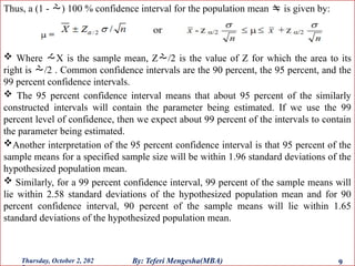
Thus, a (1 - ) 100 % confidence interval for the population mean  is given by:
 Where X is the sample mean, Z/2 is the value of Z for which the area to its
right is /2 . Common confidence intervals are the 90 percent, the 95 percent, and the
99 percent confidence intervals.
 The 95 percent confidence interval means that about 95 percent of the similarly
constructed intervals will contain the parameter being estimated. If we use the 99
percent level of confidence, then we expect about 99 percent of the intervals to contain
the parameter being estimated.
Another interpretation of the 95 percent confidence interval is that 95 percent of the
sample means for a specified sample size will be within 1.96 standard deviations of the
hypothesized population mean.
 Similarly, for a 99 percent confidence interval, 99 percent of the sample means will
lie within 2.58 standard deviations of the hypothesized population mean and for 90
percent confidence interval, 90 percent of the sample means will lie within 1.65
standard deviations of the hypothesized population mean.

If  = 0.05, then the (1 -) 100 percent confidence interval, which is the (1 – 0.05)
100 = 95 percent confidence interval and if  = 0.01, then the (1 -) 100 percent
confidence interval will be the (1 – 0.01) 100 which is the 99 percent confidence
interval. Where 1-  is called the confidence coefficient and  represent level of
error/ tolerance of error .
If  = 0.10, then Z/2= Z 0.05 = 1.65, for 90% confidence level
 The total area under the normal curve is 1. Or one can report as, 95 percent of the
area under the standard normal curve is between Z value - 1.96 and 1.96 and similarly
99 percent of the area under the standard normal curve is between Z value – 2.58 and
2.58 and between Z value- 1.65 and 1.65 and between Z value of -2.33 and 2.33 for 90
percent and 98 percent respectively.

Example 1: In a certain small city, to estimate the mean monthly expenditure for food,
a random sample of 25 households was randomly selected yielding a mean of 200 Birr.
From experience, it is known that such expenditures are normally distributed with a
standard deviation of 50 Birr.
a) What is the point estimate of the mean monthly expenditures for food of all
households in the city?
b) Find a 95 percent confidence interval for the mean monthly expenditures for food
of all households in the city.
Solution:
Given: = 200 Birr,  = 50 Birr, n = 25, and CI = 95%
c) A point estimate of the population mean  is the sample mean X,
Thus, = 200 Birr.
For 95% confidence interval, let us find .
= 1- 0.95= 0.05 Then, Z/2 = Z 0.05/2 = Z 0.025 = 1.96 (from the table of standard
normal) . Thus, a 95 % confidence interval for the mean is:

µ = x  Z/2*/n = 200  1.96 * 50/25
= 200  1.96*10= 200  19.6 = (180.40 Birr, 219.60 Birr)
 Hence, we are 95 percent confident that the true mean monthly expenditure for food
() is between 180.40 Birr and 219.60 Birr. A 95 percent Interval around the
Population Mean

Approximately 95 percent of sample means can be expected to fall within the
interval:
Conversely, about 2.5 percent can be expected to be above X+ 1.96*/n and
2.5 percent can be expected to be below X- 1.96*/n .
So 5% can be expected to fall outside the interval
Example 2: The average monthly electricity consumption for a sample of 100 families
is 1250 units. Assuming the standard deviation of electric consumption of all families is
150 units. Construct a 90 percent confidence interval estimate of the actual mean
electric consumption.
Solution: Given: = 1250,  = 150, n = 100, and Confidence Interval = 90
percent.
Z/2 = 0.10/2 = 1.65 or 1.64. Thus, confidence limits with Z/2 =  1.65 or 1.64 or
1.645.

 Thus, for 90 percent level of confidence, the populations mean µ is likely to fall
between 1225.25 units and 1274.75 units that is 1225.25 ≤ µ ≤ 1274.75.
 The quantity Z/2* /n is often called the margin of error or the sampling
error. Hence in the above example, the margin of error or the sampling error is 24.75
units.
 If a given confidence interval is given: we can calculate margin of error or the
sampling error using the formula , Upper Limit - Lower Limit / 2 , let us take the
above confidence interval 1225.25  1274.75 units; margin of error = 1274.75-
1225.25/2=49.5/2= 24.75
 Sample mean(X ) is calculated from a given interval, using :
X= lower limit of the interval + margin of error or
X= upper limit of the interval - margin of error
 Finding a specific confidence level using the inverse rule of : margin of error
Exercise 1: A normal population has a standard deviation of 10. A random sample of
size 25 has a mean of 50.
a) Construct a 90 percent confidence interval estimate of the population mean?
b) Construct a 95 percent confidence interval estimate of the population mean?
c) Construct a 98 percent confidence interval estimate of the population mean?
d) Construct a 99 percent confidence interval estimate of the population mean?

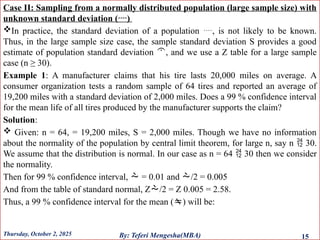
Case II: Sampling from a normally distributed population (large sample size) with
unknown standard deviation ()
In practice, the standard deviation of a population , is not likely to be known.
Thus, in the large sample size case, the sample standard deviation S provides a good
estimate of population standard deviation , and we use a Z table for a large sample
case (n ≥ 30).
Example 1: A manufacturer claims that his tire lasts 20,000 miles on average. A
consumer organization tests a random sample of 64 tires and reported an average of
19,200 miles with a standard deviation of 2,000 miles. Does a 99 % confidence interval
for the mean life of all tires produced by the manufacturer supports the claim?
Solution:
 Given: n = 64, = 19,200 miles, S = 2,000 miles. Though we have no information
about the normality of the population by central limit theorem, for large n, say n  30.
We assume that the distribution is normal. In our case as n = 64  30 then we consider
the normality.
Then for 99 % confidence interval,  = 0.01 and /2 = 0.005
And from the table of standard normal, Z/2 = Z 0.005 = 2.58.
Thus, a 99 % confidence interval for the mean () will be:

 Hence, we are 99 percent confident that the true mean mile age is at most 19,845.
Which is less than the claimed mean 20,000 miles. Therefore, the claim is not true.
Exercise 1: The wildlife department has been feeding a special food to rainbow trout
finger lings in a pound. A sample of the weight of 40 trout revealed that the mean
weight is 402.7 grams and the standard deviation 8.8 grams.
A. What is the point estimated mean weight of the population? What is that estimate
called?
B. What is the 99 percent confidence interval?
C. What are the 99 percent confidence limits?
D. Interpret your findings?

Case III: Sampling from a normally distributed population with unknown
standard deviation () and n < 30
 If the population standard deviation  is not known, then it must be estimated by
the sample standard deviation S. Under this situation, since  is estimated by S, the
sampling distribution of the mean deviates from the Normal distribution for small size,
or we say the sampling distribution follows the students t distribution with n – 1
degrees of freedom.
 For n > 30, the student t distribution can be approximated by the Normal
distribution.
Like the Normal distribution, the t-distribution is symmetrical about the mean = 0. But
it is flatter as compared to the Normal distribution.
 However, as the sample size increases the t-distribution losses its flatness and
becomes approximately Normal. The shape of the t- distribution is determined by the
degrees of freedom. Degrees of freedom can be defined as the number of values we
can choose freely.
 Generally, for a sample of size n, the degree of freedom is n – 1. The values of t for
different degrees of freedom and different values of X are tabulated. t (n – 1) denotes
the value of t for which the area under the curve to its right is equal to  with (n – 1)
degrees of freedom. The expected value of the parameter is:
 = X  t/2* Sn

Example1: A random sample of six cars from a particular model year had the following
fuel consumption figures, in miles/gallon: 18.6, 18.4, 19.2, 20.8, 19.4, and 20.5. Find a
90% confidence interval for the population mean fuel consumption for cars of this
model year, assuming that the population distribution is normal?
= 19.48 S = 1.06
n = 6, degree of freedom = 6 - 1 = 5.
t /2 = t 0.10/2 = t 0.05, 5 = 2.02 (from the t table).
= 18.61 ≤ µ ≤ 20.35
 Our 90% confidence interval for the population mean fuel consumption for these
cars ranges from 18.61 to 20.35 miles/gallon.

Example2 : The mean base salary of the judges is Birr 1800. Assume that this survey is
based on a random sample of 20 judges. Further assume that the current base salaries of
all judges have an approximate normal distribution, and the sample standard of all
judges have an approximate normal distribution, and the sample standard deviation is
Birr 500. Determine a 99% confidence interval for the population mean. What is the
point estimate?
Given: n = 20,  x= Birr 1800, s = Birr 500 and confidence level = 99% of .99
The standard deviation of (sx) =S/n = 500/20 = 500/4.472= Birr 111.81
The number of degrees of freedom, df = n -1= 20 – 1= 19
Area in each tail of the t distribution = .5 -(.99/2) = .5-.4950 = .005
 From the t distribution table, 19 degrees of freedom and .005 areas in the right tail
are 2.86. The 99% confidence interval for µ = X+ t/2*S/n
= Birr 1800 + 2.86 (111.81)
= Birr 1800 + Birr 319.78 = Birr 1480.22 – Birr 2119.78.
 Thus, we can state with 99% confidence that based on this sample the mean base
salary of all judges is between Birr 1480.22 – Birr 2119.78. Again, we can decrease the
width of a confidence interval for µ either by lowering the confidence level of by
increasing the sample size. However, increasing the sample size is the better
alternative. The point estimate = Birr 1,800.

Interval Estimation for Difference of Two Means
If all possible samples of large size n1 and n2 are drawn from two different
populations, then sampling distribution of the difference between two means x1 and x2
is approximately normal with mean (µ1-µ2 ) and standard deviation:
For a desired confidence level, the confidence interval limits for the population mean
(µ1-µ2 )are given by :
=
Illustration : The strength of the wire produced by company A has a mean of 4,500
kg and a standard deviation of 200 kg. Company B has a mean of 4000 kg and a
standard deviation of 300 kg. A sample of 50 wires of company A and 100 wires of
company B are elected at random for testing the strength. Find 99 per cent confidence
limits on the difference in the average strength of the populations of wires produced by
the two companies. Solution: The following information is given:

 Hence, the 99 percent confidence limits on the difference in the average strength of
wires produced by the two companies are likely to fall in the interval 393.80  µ 
606.20.
Confidence interval to estimate using the finite correction factor

Example : A study is conducted in a company that employs 800 engineers. A random
sample of 50 engineers reveals that the average sample age is 34.3 years. Historically,
the population standard deviation of the age of the company’s engineers is
approximately 8 years. Construct a 98% confidence interval to estimate the average age
of all the engineers in this company.
Solution
This problem has a finite population. The sample size, 50, is greater than 5% of the
population, so the finite correction factor may be helpful. In this case
N = 800, n = 50, s = 8 x = 34.30, and . The z value for a 98% confidence interval is
2.33 (.98 divided into two equal parts yields .4900; the z value is obtained from table
by using .4900).

2.3.2 Confidence Interval for the Population Proportion (P)
When np and nq are both greater than 5, and when n is large relative to the size of the
population, the approximate confidence interval for population proportion P, is given
by:
Where, ̅p = sample proportion
n = sample size
Z = Z value for degree of confidence selected
Example 1: On a certain region a sample of 500 members of the labor force showed
that 40 were unemployed. Find the 95% confidence interval for the proportion
unemployed in the region.

Example 2: Suppose 1600 of 2000 registered voters sampled said that they planned
to vote for ABC party candidate. Using the 0.95 degree of confidence, what is the
interval estimate for the population proportion?
 The quantity is often called the margin of error or the sampling error
of the proportion. Hence in the above example, the margin of error or the sampling
error proportion is 0.0176.
If a given confidence interval of the proportion is given: we can calculate margin of
error or the sampling error the proportion using the formula :
Upper Limit- Lower Limit /2 , let us take the above confidence interval 0.7824 to
0.8176 margin of error = 0.8167- 0.7824/2=0.0352/2= 0.0176

Sample proportion(̅p) calculated from a given interval, using :
̅p = lower limit of the interval + margin of error or
̅p = upper limit of the interval- margin of error
Finding a specific confidence level using the inverse use of : margin of error
Illustration : Suppose we want to estimate the proportion of families in a town, which
have two or more children. A random sample of 144 families shows that 48 families
have two or more children. Setup a 95 per cent confidence interval estimate of the
population proportion of families having two or more children.

 Hence the population proportion of families who have two or more children is likely
to be between 25.6 to 41 per cent, that is, 0.256  p  0.410.
Confidence interval estimation for the difference of two Population proportions
 There are also several situations in business where it would be necessary to estimate
the difference in two population proportions. It would be necessary to know if there is
any difference in the market share proportion of two products or it would be necessary
to know the difference in the proportion of trained workers in two different
departments of an organization.
 The procedure for constructing confidence interval estimate for the difference in two
population proportions is simply the extension of the procedure for constructing
confidence interval estimation of single proportion as follows:

Example : Consider that we have a random sample of 200 workers of an industry of
which 50 are graduates and 250 workers of a second industry 80 are graduates.
Construct a 99% confidence interval estimate for the difference in the proportion of
graduates in the two industries.
Solution

2.4 Determining the Sample Size
 Whenever we take a sample for inferential purposes, there is always a sampling
error. This sampling error is controlled by selecting a sample that is adequate in size. If
the sample size is small, then we may fail to achieve the objective of our analysis, and
if it is too large, then we waste the resources when we gather the sample.
When we estimate the population mean  by the sample mean , with probability (1 -
) the maximum error E will be:
 E = Z/2 /n if  is known
 E = Z/2 S/n if  is not known
With probability (1 - ), the sampling error will not exceed some prescribed quantity
E if the sample size is at least:
 If n comes out fractional, round up to the next integer.
n = size of the sample
Z = standard normal value corresponding to the desired level of confidence
 / S = estimate of the population standard deviation
E = maximum allowable error

Example 1: The owner of a chain of hotels wants to determine the mean number of
rooms occupied per day (so that he can have an estimate of the average daily revenue
obtained by renting rooms). From past records, the standard deviation of the daily
occupancy is known to be 9 rooms. How large a sample of days should be taken so that
the true mean number of rooms occupied per day will not differ from the sample mean
by no more than 3 rooms at the 95 percent confidence level?
Solution: Given  = 9 rooms
E = 3 rooms, (1 - ) 100 % = 95 %   = 0.05
 Z/2 = Z 0.025 = 1.96

Example 2: A certain company makes light fixtures on an assembly line. An efficiency
expert wants to determine the mean time it takes an employee to assemble the switch
on one of these fixtures. A preliminary used a random sample of 45 observations and
found that the sample standard deviation was 75 seconds. How many more
observations are necessary for the efficiency expert to be 95% sure that the point
estimate will be ''off'' from the true mean by at most 15 seconds.
Solution: Given  = S = 75 seconds
E = 15 seconds, (1 - ) 100 % = 95 %   = 0.05
 Z/2 = Z 0.025 = 1.96
 The efficiency expert should use a sample of minimum size 97. Since the
preliminary study has 45 observations, an additional of 97 - 45 = 52 observations are
necessary.

Determining Sample Size for a Population Proportion
Remember , if we do not have values for ̅p we will have to make a guess; and better to
guess P , we may set p = 0.50 in the formula for n.
Example 1: A market research firm wants to estimate the proportion of households in a
certain area that have color television sets. The firm would like to estimate P to within
0.05 with 95% confidence. No estimate of P is available. Determine the sample size.
Solution: Given E = 0.05, p = 0.50 (because no better estimate is available), q = 0.50
(1 - ) 100 % = 95 %   = 0.05
 Z/2 = Z 0.025 = 1.96

Example 2: A survey was conducted to know the proportion of consumers who buy a
newly produced soap. The study wanted to be 99% confident that the estimate is within
 2% of the true population proportion. What sample size should be taken if a
previous survey showed that 40% of consumers buy it?
Solution : For 99% level of confidence, the value of Z0.01/2 = Z 0.005 = 2.58.
P = 0.4, E = 0.02 then,
Therefore, the sample size that must be taken is 3994consumers
Example 3: ABC manufacturing company wants to estimate the proportion of parts
produced by the new machine that are defective. The company manager wants this
estimate to be within .02 of the population proportion for a 95% confidence level. What
is the most conservation estimate of the sample size that will limit the maximum error
to be within .02 of the population proportion?
 The required sample size (n) = (z/2)2
p q = (1.96)2
(.50) (.50) = 2401
E2
(.02)2
Thus, if company takes a sample of 2401 parts, the estimate of P will be within .02 of
the population proportion.

Summary of Confidence Interval for µ

Exercise:
1. For a population data, σ = 16.42
a) What should the sample size be for a 98% confidence interval for µ to have a
maximum error of estimate equal to 5.5?
b) What should the sample size be for a 95% confidence interval for µ to have a
maximum error of estimate equal to 4.25?
2. A researcher wants to determine a 95% confidence interval for the mean number of
hours that college students spend doing homework per week. He knows that the
standard deviation for hours spent per week by all college students doing homework is
12. How large a sample should the researcher select so that the estimate will be within
2 hrs of the population mean?
3. Suppose a preliminary study was conducted on the number of kilo meters that
residents travel on a day. Assume that the population standard deviation is 8 kilo
meters and the confidence level is 95%. What sample size of residents should be
selected for a study to estimate the mean number of kilo meters that the residents travel
per day in a car to be within + 2 kilo meters?

4. A sales manager wants to estimate at a 90% confidence level that the mean amount
of money spent by all customers at its store. From an earlier study, the manager
knows that the standard deviation of amounts spent by customers at this store is
Birr 30. What sample size should he choose so that the estimate is within Birr 4 of
the population mean?
5. Assume that a preliminary study has shown that 76% of drivers wear seat belts while
driving. How large should the sample size be so that the 99% confidence interval for
the population proportion has a maximum error of .03?
6. Find the most conservative sample size that will produce the maximum error for a
98% confidence interval for p (E) = .045.
7. A company has 10,000 workers. To estimate the average income per month of these
workers, a random sample of 600 workers are chosen and found average income of
Birr 800 per month with standard deviation of Birr 150. Construct a 95% confidence
interval for the average income per month of all workers.
8. Suppose that a study showed that a sample of 150 professional working men earn
average monthly salary of Birr 30,000 with standard deviation of Birr 800 and a
sample of 100 professional working women earn monthly salary of Birr 25,000 with
standard deviation of Birr 600. Assuming that salary is normal, construct a 99%
confidence interval estimate for the difference in average salary between professional
working men and professional working women.

THE END
THANK YOU

Chapter two statistics stat au university 2.pptx

More Related Content

Similar to Chapter two statistics stat au university 2.pptx

Recently uploaded

Chapter two statistics stat au university 2.pptx