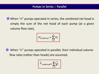
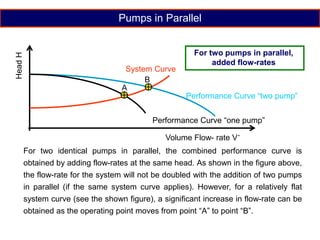
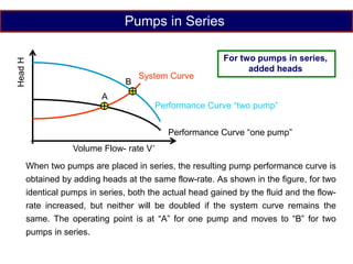
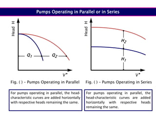
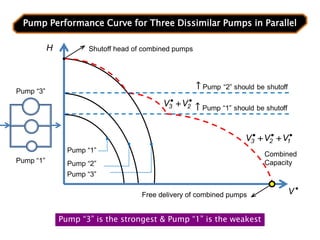
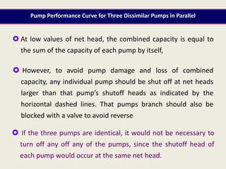
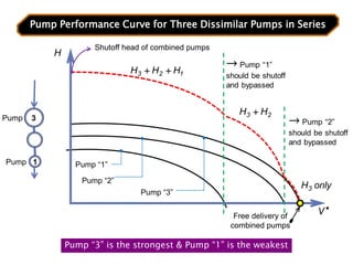
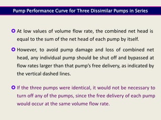
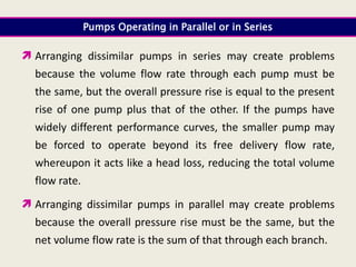
Performance curve.ppt

 When faced with the need to increase volume flow rate or pressure
rise by a small amount, we might consider adding an additional small
pump in parallel or in series with the original pump.
 However, to avoid pump damage and loss of combined capacity, any
individual pump should be shutoff at net heads larger than that that
pump’s shutoff heads as indicated by the horizontal dashed lines.
That pump’s branch should also be blocked with a valve to avoid
reverse flow.
Pumps in Parallel and in Series
 If the three pumps are identical, it would not be necessary to turn
off any off of the pumps, since the shutoff head of each pump would
occur at the same net head.

A pump head-characteristic curve is a graphical representation of the
total head versus the discharge that a pump can supply. These curves, which
are determined from pump tests, are supplied by the pump manufacturer.
Two points of interest on the pump curve are the shutoff head and the
normal discharge or rated capacity.
 The shutoff head is the head output by the pump at zero discharge,
while the normal discharge (or head) or rated capacity is the discharge
(or head) where the pump is operating at its most efficient
 Variable speed motors can drive pumps at a series of rotative speeds,
which would result in a set of pump curves for the single pump, as
illustrated in the following curve.
Definitions

Flow Rates
₪ Volume flow rate: is the volume of fluid flowing past a
section per unit time.
₪ Mass flow rate: is the mass of fluid flowing past a
₪ Weight flow rate: is the weight of fluid flowing past a



Pump hS
Flow rate
Head
System-head-capacity Curve with Negative Lift
The figure illustrates a system-head-
curve with a negative lift.

Friction, Fitting,
and Valve Losses


Pump
hS
Total Static Head
Flow rate
Head
System-head-capacity Curve with Positive Lift
curve in which the head is the sum of
friction, fitting, and valve losses.
curve in which the head is the sum of
friction, fitting, and valve losses.

For Max. Lift
For Min. Lift
Flow rate
Head
System-head-capacity Curve with Varying Static Lift
Z (max)
Z (min)


Pump
hS (min)

hS (max)
hS (max)
hS (min)
curve with a varying static lift. One for
the minimum lift and the second for
the maximum

System Throttled by Valve Operation


Valve
Flow rate
Head
The figure illustrates a system-head-curve
for a throttled system in which various
valve opening are used to vary the head-
discharge curve.

 When “n” pumps operated in series, the combined net head is
simply the sum of the net head of each pump (at a given
volume flow rate),
Pumps in Series / Parallel



n
1
i
i
combined H
H
 When “n” pumps operated in parallel, their individual volume
flow rates (rather than heads) are assumed,




 n
1
i
i
combined V
V

Pumps Operating in Parallel or in Series
 Pump manufacturers also provide curves relating to the break
horsepower (required by pump) to the pump discharge. The break
horsepower is calculating using
550
H
Q
g
bhp
e 



Where:
Q is the pump discharge in cfs,
H is the total head in ft,
.g is the specific weight of water
in Ib / ft3, and
e is the pump efficiency.
Where:
Q is the pump discharge in m3/s,
H is the total head in m,
.g is the specific weight of water in
kilonewtons/m3, and
e is the pump efficiency.
e
H
Q
g
bhp



The break horse power (bhp) The (bhp) in SI unites is given in
kilowatts

Pumps in Parallel
Volume Flow- rate V
.
Performance Curve “one pump”
Performance Curve “two pump”
System Curve
A
B
Head
H
For two identical pumps in parallel, the combined performance curve is
obtained by adding flow-rates at the same head. As shown in the figure above,
the flow-rate for the system will not be doubled with the addition of two pumps
in parallel (if the same system curve applies). However, for a relatively flat
system curve (see the shown figure), a significant increase in flow-rate can be
obtained as the operating point moves from point “A” to point “B”.
For two pumps in parallel,
added flow-rates

Pumps in Series
Volume Flow- rate V
.
Performance Curve “one pump”
Performance Curve “two pump”
System Curve
A
B
Head
H
When two pumps are placed in series, the resulting pump performance curve is
obtained by adding heads at the same flow-rate. As shown in the figure, for two
identical pumps in series, both the actual head gained by the fluid and the flow-
rate increased, but neither will be doubled if the system curve remains the
same. The operating point is at “A” for one pump and moves to “B” for two
pumps in series.
For two pumps in series,
added heads


V
Head
H
Fig. ( ) – Pumps Operating in Parallel
Q1 Q2

V
Head
H
H1
H2
Fig. ( ) – Pumps Operating in Series
For pumps operating in parallel, the head-
characteristic curves are added horizontally
with respective heads remaining the same.
For pumps operating in parallel, the
head-characteristic curves are added
horizontally with respective heads
remaining the same.


V
Head
H
500 rev/min
800 rev/min
1000 rev/min
1200 rev/min
Fig. ( ) - Pump Performance Curves for Variable-speed Pumps.
Pump Performance Curves for Variable-speed Pumps.

A better course of action is to
 Increase the original pumps speed and/or input power
(large electric motor),
 Replace the impeller with a larger one, or
 Replace the enter pump with a larger one.

hS
System Head Curve
Pump Characteristic Curve
Volume Flow Rate
Efficiency
Head
Efficiency
Determination of Operating Points for a Single Speed Pump
For a Fixed Static Lift (head) hS

Determination of Operating Points for a Single Speed Pump
 In order to determine the operating point for a pump or
pumps in a piping system, the characteristic curve is
superimposed on the system curve as illustrated in the figure.
 The point of intersection of the two curves is the pump
operating point.
 The pump operating point should be at or near the maximum
efficiency of the

hS Max.
Characteristic Curve for
two Pumps
Volume Flow Rate
Head
Determination of Operating Points for Two Single Speed Pumps
Pumps in Parallel and a Variable Static Lift (head) hS
Characteristic Curve for
one Pump
hS Min.
Maximum System Curve
Minimum System Curve
Operating Points
Possible range of
operation for one pump
Possible range of
operation for two pumps

Determination of Operating Points for Two Single Speed Pumps
 The figure illustrates the operating points for two single-
speed pumps operating in parallel for piping system that has
a range of static lift
 The system curves are shown for the maximum lift and the
minimum lift.
 Also shown is the range of operating points (between
minimum and maximum static lift) for a single pump.


V
Head
H
100% speed
System with a Single Pump Operating at Variable-speed
95% speed
90% speed
85% speed
Operating Points
hS
System Curve
 The Figure illustrates the operating points for a variable-speed pump
with a system curve. The affinity laws can be used to determine the
rotational at any desired operating points.

Pump “1”
Pump “2”
Pump “3”
Combined
Capacity
Shutoff head of combined pumps
Free delivery of combined pumps
Pump Performance Curve for Three Dissimilar Pumps in Parallel
Pump “3” is the strongest & Pump “1” is the weakest
Pump “3”
Pump “1”

V


 2
3 V
V




 1
2
3 V
V
V
H

 At low values of net head, the combined capacity is equal to
the sum of the capacity of each pump by itself,
 However, to avoid pump damage and loss of combined
capacity, any individual pump should be shut off at net heads
larger than that pump’s shutoff heads as indicated by the
horizontal dashed lines. That pumps branch should also be
blocked with a valve to avoid reverse
 If the three pumps are identical, it would not be necessary to
turn off any off any of the pumps, since the shutoff head of
each pump would occur at the same net head.
Pump Performance Curve for Three Dissimilar Pumps in Parallel

Pump “1”
Pump “2”
Pump “3”
Shutoff head of combined pumps
Free delivery of
combined pumps
Pump Performance Curve for Three Dissimilar Pumps in Series
Pump “3” is the strongest & Pump “1” is the weakest
Pump 3
Pump 1
H
1
2
3 H
H
H 

2
3 H
H 
only
H3

V

 At low values of volume flow rate, the combined net head is
equal to the sum of the net head of each pump by itself.
 However, to avoid pump damage and loss of combined net
head, any individual pump should be shut off and bypassed at
flow rates larger than that pump’s free delivery, as indicated by
the vertical dashed lines.
 If the three pumps were identical, it would not be necessary to
turn off any of the pumps, since the free delivery of each pump
would occur at the same volume flow rate.
Pump Performance Curve for Three Dissimilar Pumps in Series

 Arranging dissimilar pumps in series may create problems
because the volume flow rate through each pump must be
the same, but the overall pressure rise is equal to the present
rise of one pump plus that of the other. If the pumps have
widely different performance curves, the smaller pump may
be forced to operate beyond its free delivery flow rate,
whereupon it acts like a head loss, reducing the total volume
flow rate.
 Arranging dissimilar pumps in parallel may create problems
because the overall pressure rise must be the same, but the
net volume flow rate is the sum of that through each branch.

Operating Characteristics
 Operating characteristics of pumps are dependent upon their:
 Size  Speed  and design
 In centrifugal pumps, similar flow patterns occur in geometrically
similar pumps. Through dimensional analysis the following three
independent coefficients can be derived to describe the operation
of pumps.
3
Q
D
N
Q
C
:
t
coefficien
Discharge
- 
2
2
H
D
N
H
C
:
t
coefficien
Head
- 
ess)
correction
l
dimensiona
(for
D
N
H
g
C
or 2
2
H 
5
3
H
D
N
P
C
:
t
coefficien
Power
-


Affinity laws
Even though it is not dimensionally
correct, it is commonly used

3
1
2
1
2
1
2










D
D
N
N
Q
Q
2
1
2
2
1
2
1
2


















D
D
N
N
H
H
5
1
2
3
1
2
1
2
1
2



















D
D
N
N
P
P


 If pump “1” and pump “2” are from the same geometric family and
are operating at homologous points (the same dimensionless
position), their flow rates, heads, and powers will be related as
follows:
These are the similarity
rules, which can be used to
estimate the effect of
changing the fluid, speed,
or size on any dynamic
turbo machine-pump or
turbine within a
geometrically similar family

 These equations are the same either in SI of BG units, but with
different values.
ft3/s
m3/s
is pump capacity
Q
r.p.m
radians /
second
is the speed
N
ft
m
is the impeller diameter
D
32.2ft3/s
9.81m3/s
is the acceleration due to gravity
g
horsepower
kilowatts
is the power
P
Slugs/ft3
Kg/m3
is the density


 The coefficients mentioned before can be used to define the
affinity laws for a pump operating at two different speeds and the
same diameter. Consider the ratios (CQ)1 = (CQ)2 for the same
diameter and different speeds N1 and N2. (where 1 and 2 represent
corresponding points)
2
1
2
1
N
N
Q
Q

Similarly for (CH)1= (CH)2:
2
2
1
2
1
N
N
H
H









and similarly for (CP)1= (CP)2:
3
2
1
2
1
N
N
P
P









Affinity laws for
discharge and for head
equation are accurate
The affinity laws for power
may not be accurate

 These relationships assume that the efficiency remains the same
for one point on a pump curve to a homologous point on another
pump curve.

Specific Speed “NS”
 The specific speed NS is not really representative of any meaningful
or measurable speed in a machine, so some practitioners refer to it
as “type number”, since it is used in selection of pump type.
 The value of NS for a particular machine is calculated for the
conditions obtained at its point of optimum efficiency, since ideally
this should coincide with the installed operating point of pump.
 The wide variety of units are used in calculating values of NS. The
engineer needs to check this point carefully with the pump
manufacturer.

3
Q
D
N
Q
C  2
2
H
D
N
H
C 
can be eliminated by dividing CQ
1/2 by CH
1/2 as so the specific
speed becomes
H
Q
N
)
D
N
H
(
)
ND
Q
(
C
C
N 4
3
4
3
2
2
2
1
3
4
3
H
2
1
Q
S 


The discharge and head coefficients
Historically the “g”
term was disregarded
4
3
2
1
4
3 /
/
S
ft
min)
/
gal
(
)
m
.
p
.
r
(
H
Q
N
N



Note:
NS is applied
only to BEP
Best Efficient
Point

a very rough guide to the range of duties covered by the different
machine is as follows:
Taking
N: revolution/ min Q: in m3/s and H: in m
 10 ˂ NS ˂ 70 : centrifugal pump (high head, low to moderate discharge)
 70 ˂ NS ˂ 165 : mixed flow pump (moderate head, moderate discharge)
 NS ˂ 165 : axial flow pump (low head, high discharge)

Worked Example
 A 6.85-in pump, running at 3500 r.p.m, has the following measured
performance for water:
450
400
350
300
250
200
150
100
50
Q,
(gal/min)
139
156
169
181
189
194
198
200
201
H ( ft)
74
79
81
80
77
72
64
50
29
 %
A. Estimate the horsepower at BEP.
B. If this pump is rescaled in water to provide 20hp at
3000 r.p.m, determine the appropriate:
C. Impeller diameter,
D. Flow rate, and
E. Efficiency for this new condition.

  hp
.
.
.
)
.
.
(
/
H
Q
g
power 47
18
550
81
0
169
10
228
2
350
2
32
94
1 3













Worked Example
From the table given:  at best efficient point = 81% and the
corresponding flow rate = 350 gal/min and the head = 169 ft. The
corresponding horsepower
N = 3000 r.p.m
N = 3500 r.p.m
D2 = ??-in
D1 = 6.85-in
Q2 = ??? gal/min
Q1 = 350 gal/min
(Power) 2 = 20 hp
(Power) 1 = 18.47 hp
The given data can be tabulated in the following table:

3
1
2
1
2
1
2










D
D
N
N
Q
Q
Worked Example
Applying the similarity laws:
gives
min
/
gal
.
.
D
D
N
N
Q
Q 415
85
6
63
7
3000
3500
350
3
3
1
2
1
2
1
2 





















5
1
2
3
1
2
1
2
1
2



















D
D
N
N
P
P

 gives
5
2
3
85
6
3500
3000
47
18
20














.
D
.
 which gives in
.
D 
 63
7
2
The efficiency for this new condition have to be = 81%:

Worked Example
 Tests on a 14.62-in-diameter centrifugal water pump at 2134 r.p.m
yields the following data:
10
8
6
4
2
0
Q, (ft3/sec)
220
300
330
340
340
340
H ( ft)
330
330
255
205
160
135
bhp
A. What is the BEP?
B. What is the specific speed?
C. Estimate the maximum discharge possible.
Table (1)


 /
H
Q
g
power
horse
break 

Worked Example
550
2
32
94
1
H
Q
.
.
bhp
/
H
Q
g
or




 

 Substituting the given values (Table 1) into Eq. (1) for 2134 r.p.m
gives :
10
8
6
4
2
0
Q, (ft3/sec)
220
300
330
340
340
340
H ( ft)
330
330
255
205
160
135
bhp
76
83
88
75
48
0
 %
1.0 gallon/min=
2.22810-3 ft3 / sec
……………….….. (1)

4
3
2
1
4
3 /
/
S
ft
min)
/
gal
(
)
m
.
p
.
r
(
H
Q
N
N



sec
/
ft
.
.
3
3
3
10
69
2
10
228
2
6
gal./min
in
Q 


 

The specific speed NS can be determined using
Worked Example
1430
330
10
69
2
2134
4
3
2
1
3
4
3





 /
/
S
)
(
)
.
(
H
Q
N
N

 /
H
Q
g
power
horse
break 

s
/
ft
.
.
H
g
Q
3
6
330
2
32
94
1
550
88
255
550
power
horse
break













Z (max)
Z (min)


Pump
hS (min)

hS (max)

 3 to 4ycr
ycr
ycr
Example Locations of Critical Flow
Critical Depth near Overfall
Flow over a Broad-crested Weir

ycr
Hydraulic Jump

Flow Through a Hydraulic Jump
ycr
Chang in the Bottom Slope of the Channel

 3 to 4ycr
ycr
ycr
Example Locations of Critic
 3 to 4ycr
ycr
ycr
Example Locations of Critical Flo
ycr
Hydraulic Jump

ycr
ycr
Hydraulic Jump

ycr

hp
EGL
Z1- Zo
Zo=0
P0 = 14.7 psi
P0/g = 34ft
EGL
Pv = 0.506 psi
Pv/g = 1.17ft
For water at T=27oC

L
V
Valve
Reservoir
Hydraulic Grade Line
Static Pressure Line
Surge Pressure Line
(a)
(b)
(a) Pipeline System,
(b) Surge Pressure at Valve.

f1 & D1 & L1
f2 & D2 & L2 f3 & D3 & L3


  
EGL
B
A



 L
h
H
B
A

Q Q
F2 & D2 & L2 & Q2
A B
F1 & D1 & L1 & Q1


10 ft
2 ft
3 in
1 in
h
Water
Mercury


 mercury"
"
liquid
indicating
the
in
Z
Z
at
P
P 4
3
4
3 


1.0m
1.5m
1.2m
pump








R = 0.6m
 
3.0m
A
A
Sec. A-A
30o

Expansion Joints
Concrete Anchors
Bend
30o

P1
P2
V1
V2
y
x
The general momentum equation
for steady one-dimensional flow
is:
30o
The continuity equation gives:
A pipe has a 30o horizontal bend in it

Control Surface




A Fitting between Two Pipes of Different Size (TRANSITION)
The continuity equation gives:
The general momentum equation
for steady one-dimensional flow
is:
x
y
P1
V1 V2
P2
)
V
V
(
Q
F
p
p
1
2
bold
2
1






P3
P2
P1
x
y
s
c
B
A
x
y
z

Crest Level
 Water Level
B
dh
H
h

Performance curve.ppt

More Related Content

What's hot

Similar to Performance curve.ppt

More from Dr. Ezzat Elsayed Gomaa

Recently uploaded

Performance curve.ppt