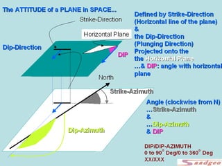
The document discusses enhanced reservoir characterization using borehole images and dipmeter data. It begins with an overview of how logging tools have advanced from single measurements to detailed mapping of borehole walls using modern imaging tools with hundreds of thousands of data points per meter. The main topics covered include different types of dipmeter and imaging tools, generating borehole maps for orientation, stereographic projections for analyzing dip distributions, and processing raw data into geologically interpretable outputs like image and dip logs. Overall, the document outlines the transition from traditional well logging to digital geological mapping using high-resolution borehole wall data.

1. ENHANCED RESERVOIR
CHARACTERISATION
BASED UPON
BOREHOLE
IMAGES SAADALLAH GEOCONSULTANT AS
A. SAADALLAH Dr.
& Misjonsveien 39, N-4024 Stavanger Norway
Tel. + (47) 51 52 62 65 (office)
DIPMETER Email: kader@saadgeo.com
website: www.saadgeo.com
DATA

2. WARNING !
THIS PRESENTATION WAS
PREPARED IN 2005
IT HAS TO BE UPDATED BY
INCLUDING NEW TOOLS (such as
those of Weatherford) AND OTHER
ELEMENTS OF INTERPRETAION

3. ENHANCED RESERVOIR
CHARACTERISATION BASED UPON
BOREHOLE IMAGES & DIPMETER
DATA
OVERVIEW

4. 1 Introduction
2 Dipmeter Tools
3 Imaging Tools
4 Borehole Map
5 Stereographic Projections
6 From Raw Data to Geologically Interpretable Outputs
7 Basic Interpretation
8 Clastic Reservoirs
9 In Situ Stress Issue
10 Fractured Reservoirs
11 Key Features to keep in mind
12 Key References

5. INTRODUCTION

6. From Logging & Petrophysic
point of view
to
a Geologic Mapping of the
Borehole Wall concept

7. From Logging & Petrophysic point of view to a Geologic
Mapping of the Borehole Wall concept
Curve:
ONE value (Rock Propriety)
vs.
ONE Depth (MD)

8. From Logging & Petrophysic point of view to a Geologic
Mapping of the Borehole Wall concept
Curve: a value (Rock Propriety) vs. Depth (MD)
Dip needed very early in
Logging industry (Seismic not
yet performed or/and poor, Oil
goes up!)

9. From Logging & Petrophysic point of view to a Geologic
Mapping of the Borehole Wall concept
Curve: a value (Rock Propriety) vs. Depth (MD)
Dip needed very early in Logging industry (Seismic not yet
performed or/and poor, Oil goes up!)
Dip needs a set of at least 3
measurements of the SAME
FEATURE: Dipmeter tool: 4
curves

10. From Logging & Petrophysic point of view to a Geologic Mapping of
the Borehole Wall concept
Curve: a value (Rock Propriety) vs. Depth (MD)
Dip needed very early in Logging industry (Seismic not yet
performed or/and poor, Oil goes up!)
Dip needs a set of at least 3 measurements of the SAME FEATURE:
Dipmeter tool: 4 curves
Technology improvements: more data,
magnetometers, accelerometers, transmission
of data (pulse within mud) IMAGING
TOOLS: ca 100 000 measurements per Meter
MD: MAPPING OF THE BOREHOLE
WALL.

11. From Logging & Petrophysic point of view to a
Geologic Mapping of the Borehole Wall concept
Curve: a value (Rock Propriety) vs. Depth (MD)
Dip needed very early in Logging industry (Seismic
not yet performed or/and poor, Oil goes up!)
Dip needs a set of at least 3 measurements of the
SAME FEATURE: Dipmeter tool: 4 curves
Technology improvements: more data,
magnetometers, accelerometers, transmission of
data (pulse within mud) IMAGING TOOLS: 100
000 measurements per Meter MD: MAPPING OF
THE BOREHOLE WALL.

14. From1 Dip in 1 day (1969
Sidi Ferruch Algiers)

15. 1250 Dips measured (2004) a fractured reservoir

16. From 1 Dip in 1 day (1969
Sidi Ferruch Algiers)
To
1250 Dips measured (2004
fractured reservoir)

17. From FEW to
THOUSANDS of
MEASUREMENTS
That’s
DIGITAL GEOLOGY

18. New ways of thinking,
managing data, processing,
interpreting…and more
and more data…in real
time …new challenges for
geoscientists

19. Logging History Mile Stones: 1927
Figure 1.The first electric
log was obtained Sept.
27, 1927, on the
Diefenbach 2905 well,
Rig.No. 7,
at Pechelbronn,Alsace,
France.The resistivity
curve
was created by plotting
successive readings.

20. Logging History Mile Stones: 1947
1941: logging took another major step forward with the
introduction of the Spontaneous-Potential
Dipmeter.
1947: This measurement was improved further with the
Resistivity Dipmeter
1952: Continuous Resistivity Dipmeter

21. Logging History Mile Stones:
Imaging Tools
1968 BHTV (BoreHole TeleViewer) Mobil Acoustic...
1986: FMS (Formation MicroScanner) Schlumberger Electric...
1991 FMI (Fullbore Formation Microscanner) Schlumberger...
1994 RAB (Resistivity at the Bit) LWD Schlumberger...
2001 OBMI (Oil Base MicroImager) Schlumberger...
NEXT: high resolution imaging LWD tools (technical issue to
transmit data while drilling solved: WO (2007??)
Followed by other logging companies: Baker Hughes, Halliburton

22. MAIN DIPMETER TOOLS
Logging Company
Main Technical
Tool Name Resolution Name & Mud
Characteristics
Environment
SHDT 8 microresistivity electrodes on
Schlumberger’s tool
(Stratigraphi 4 pads (2 per pads)
Water-base mud
c Dipmeter) Sampling: 0.1 in
HEXDIP Vertical
6 microresistivity electrodes on Baker Hughes’ tool
(Hexagonal resolution: 1-2
6 pads Water-base mud
Diplog) cm
SED (Six
6 microresistivity electrodes on Halliburton’ tool
Arm
6 pads Water-base mud
Dipmeter)

23. TOOL Example:
SED (Halliburton)

24. HIGH RESOLUTION IMAGING TOOLS
Electrical and Acoustic
of the main logging companies
in petroleum industry
BAKER HUGHES:
- STAR (electrical & acoustic)
- CBIL
HALLIBURTON:
- XRMI (EMI)
- CAST
SCHLUMBERGER:
- FMI (FMS)
- UBI

25. Main Characteristics of Electrical Imaging Tools
Use electrical responses of the formation to create Images.
Pad-based Microresistivity (conduct. mud),
sensitive to poor pad contact. Depth of investigation: 1 in.
Resolution linked with electrical contrast:
Bedding ca. 1 cm; Fracture ca. 1 mm (Resistivity Contrast)
EMI FMI STAR
6 Pads, 2 rows 4 Pads & Flaps 6 Pads
Arm configuration 2 X 12 Sensors 2 X 12 Sensors
25 Sensors
Sensors 150 192 144
Coverage 58% of 8.5” 75% of 8.5” 56% of 8.5”
Logging Speed 1800 ft/hr 1800/1500 ft/hr 1200/2400 ft/hr
X-, Y-Spacing 0.2 in. 0.1-0.2 in. 0.1 in.

26. Main Characteristics of Acoustic Imaging Tools
Acoustic response of the formation to build up images
Rotating transducer (Transmitter-Receiver)
Ultras. pulse 250-500 kHz. Water- and Oil-based mud,
100% borehole coverage, sensitive to borehole shape,
Depth of investigation: 0, Travel Time and Amplitude Attenuation
Resolve feature down to 1 in.
CAST UBI CBIL
200 samples/rev 7.5 Rot /Sec 6 Rot/Sec
Measurements 180 samples /rev 12 (STAR)
250 samples/rev
1 in. 2100 ft/hr
Vertical Sampling 0.3 in 0.4 in 800 ft/hr 0.2 in
rate & Logg. speed 1200 ft/hr 0.2 in 400 ft hr 2400 ft/hr
Image Resolution 0.4 in at 250 kHz
0.2 in at 500 kHz

27. TOOL Example:
FMI (Schlumberger)

28. BOREHOLE MAP

29. BoreHoleMap
Borehole
Tool
Projection: Boreholemap
Tool within the Borehole: RB
Attitude of a plane in Space
Attitude of an axis in Space
Boreholemap representation: Sinecurve
Tadpole

30. BoreHoleMap: Orientation
Borehole Axis
DEVI: Deviation (inclination): Angle 00-90 Deg (from vertical to horizontal axis)
HAZI: Borehole axis azimuth: Angle 000-360 Deg (from N-000- to N -360 clockwise)
MD: Measured Depth
Tool Axis (Sonde Axis)
DEVI: Sonde Deviation: Angle 00-90 Deg (from vertical to horizontal axis)
Sonde DEVI = Borehole DEVI
P1AZ: Ref PAD (PAD1): Azimuth PAD1 = Angle 000-360 Deg from North (000) or
from the BOREHOLE HIGH SIDE clockwise
MD: Measured Depth

33. ORIENTATION of the BOREHOLE MAP
Y-AXIS:
- Borehole High Side 0 90 180 270 3600
- Tool Frame
Y-Axis: MD
- North
& MD
X- AXIS:
- Borehole Perimeter
& Azimuthal X-Axis: Azimuthal & Perimeter

34. ORIENTATION of the
TOOL WITHIN the Borehole
Tool ROTATES (around the AXIS) its
EXACT position INSIDE the BOREHOLE
has to be known at EVERY measurement
RB: Relative Bearing:
Angle between the referenced-arm (P1AZ) and a fixed feature
(North, High side of the Borehole) is recorded at
every measured point

37. AXIS ATTITUDE in SPACE:
Dip/Dip-Azimuth

38. Core Goniometry
Methodology
1. - Projection of core-features
onto a borehole map
2. - Projection of a planar-feature
onto the borehole map (Fault…)
3. - Projection of a linear-feature of a surface
onto the borehole map
(Striation on Fault-Surface)

39. Projection of Core: Borehole Map
Orthogonal projection onto
a cylindrical surface = Borehole Map
A reference line parallel
to the core axis
= master calibration line
with the MD
= Y-Axis
Perimeter
=2PR
= 3600
= X-Axis (cm & Deg)

40. Projection of a Planar-feature
PR
DIP-AZIMUTH
Sine curve TOP PR
Sine curve BOTTOM
=DIP-AZIMUTH
Perimeter
=3600 900 1800 2700 360-00
=2PR PR/2 PR 3PR/2 2P R-0 cm
DIP-AZIMUTH (cm or Deg)
relative to the master calibration line
Master Calibration Line

41. Projection of a Planar-feature
DIP
Sine Curve
Amplitude
DZ
900 1800 2700 360-00
PR/2 PR 3PR/2 2P R-0 cm
DZ
Tang DIP =
Core Diameter

42. AXIS On Borehole Map
Fault Surface with Striation (Sandstone clast) in Shale

43. Projection of a Linear-feature
of a Surface onto the Borehole Map
PR
DZ
900 1800 2700 360-00
PR/2 PR 3PR/2
Tang DIP = DZ 2P R-0 cm
Diameter of the Core
DIP-AZIMUTH of the line relative
to the master calibration line

44. Projection of a Linear-feature
of a Surface onto the Borehole Map
900 1800 2700 360-00
PR/2 PR 3PR/2
2P R-0 cm
DIP-AZIMUTH of the LINE relative
to the master calibration line

46. N (000Deg)
TADPOLE
0 Deg 90 Deg
10/135 Deg
W (270 Deg) E (090 Deg)
15/225 Deg
S (180 Deg)

47. STEREOGRAPHIC
PROJECTION

48. We are dealing
with DIP POPULATIONS
NOT with
INDIVIDUAL DIP

49. Analysing Dip Populations:
Stereographic Projections
SCHMIDT PROJECTION
Upper Hemisphere

50. Only ORIENTATION Matters
NOT the Spatial POSITION

51. UPPER HEMISPHERE

52. Vertical & Horizontal lines

53. Girdle of Lines

54. Vertical &
Horizontal
Planes

55. One Pop. Dipping
increasingly South:
GIRDLE

56. Schmidt
Net
Lines

57. Projection of a
Plane: Pole &
Cyclographic

58. Schmidt Net
Planes

59. Schmidt Net

60. Unimodal
Population

61. Unimodal Population

62. Bimodal
Population

63. GIRDLE: Population Related to Fault

64. GIRDLE: FOLD

65. Compass Rose
360/0
348.75 011.25
326.25 033.75
045
N-S
315
.S W
N..N
NN
056.25
E-S
W-
W-
N.N
SW
S..S
303.75 NW
-S E-
EE
E N
W.
NW .SW 078.75
281.25 -E. E-W
SE E. N
270 E-W E-W 090
W.
W NW
258.75 W. S -E.
E. NE- SE 101.25
NW
N..N
NN
.SW
SW -S
E
E- 123.75
W-
W-S
N
E -S
236.25
S..SE
N.N
S
135
225 N-S
146.25
213.75 168.75
191.25
180
Dipping Striking Dipping Striking
348.75…011.25: N E-W 168.75…191.25: S E-W
011.25…033.75: N.NE W.NW-E.SE 191.25…213.75: S.SW W.NW-E.SE
033.75…056.25: NE NW-SE 213.75…236.25: SW NW-SE
056.25…078.75: E.NE N.NW-S.SE 236.25…258.75: W.SW N.NW-S.SE
078.75…101.25: E N-S 258.75…281.25: W N-S
101.25…123.75: E.SE N.NE-S.SW 281.25…303.75: W.NW N.NE-S.SW
123.75…146.25: SE NE-SW 303.75…326.25: NW NE-SW
146.25…168.75: S.SE E.NE-W.SW 326.25…348.75: N.NW E.NE-W.SW
168.75…191.25: S E-W 348.75…011.25: N E-W

66. From RAW Data to
GEOLOGICALLY
Interpretable Outputs

67. Main Processes
Raw data, microresistivity measurements recorded by electrode tool,
need to be processed:
Speed correction,
Magnetic declination correction,
Depth shift offset (when it is needed)
Generation of image/dip logs.

68. Main Processes
Speed correction,
convert data, recorded vs. time into data vs. depth
&
correct depth offset due to oscillations along the axis tool.
Oscillations are caused by irregularities of the borehole or in fact due
to the none-constant speed of the tool while running the logs.
Generally, a sliding window of 10 ft is used for an average cable speed
of 1600 ft/hr.

69. SPEED CORRECTION: is applied
to correct for erratic tool motion
& convert data recorded in time to depth
0 90 180 270 3600
T8
T3
0.2 in.
T2 T2-7
2-7
T1 T1
Y Axis: MD
T0 T0
IN THEORY: Tool moves up the IN REALITY: Tool moves ERRATICALLY up
borehole recording measurement-sets the borehole recording measurement-sets at
At regular timing (T0 – T3) regular timing (T0 – T3)

70. Main Processes
Magnetic declination correction,
applied to inclinometry measurements
recorded by the tool (relatively to the
magnetic North) to convert them to
Geographic North.

71. Main Processes
Depth shift offset (when it is needed)
Correlation of GR from another Run (Wireline Log) & GR from FMI
Geological Feature determined from other sources

72. Main Processes
Generation of images
Static normalised images (called Static Images):
computation carried out in a window covering all the
logged section.
Dynamically normalised images (called Dynamic Images):
sliding window (5 Ft).
Scale in the range white-yellow-brown-dark :
white-yellow: minimum conductivity
To
brown-dark: maximum conductivity.

73. QC: Depth Match, Static & Dynamic Images
Geological Features: Bed Boundary, Bedding

74. QC: Depth Match, Static & Dynamic Images
Geological Features: Bed Boundary, Bedding
Dynamic Image

75. QC: Depth Match, Static & Dynamic Images
Geological Features: Bed Boundary, Bedding
Static Image Dynamic Image

76. QC: Depth Match, Static & Dynamic Images
Geological Features: Bed Boundary, Bedding
Static Image Dynamic Image
Calipers

77. QC: Depth Match, Static & Dynamic Images
Geological Features: Bed Boundary, Bedding
Static Image Dynamic Image
GR
Calipers

78. QC: Depth Match, Static & Dynamic Images
Geological Features: Bed Boundary, Bedding
Static Image Dynamic Image
GR
Calipers
RHOB

79. QC: Depth Match, Static & Dynamic Images
Geological Features: Bed Boundary, Bedding
Static Image Dynamic Image
GR
Calipers
RHOB
NPHI

80. PROCESSING of
DIPMETER
DATA

81. Measurements
recorded by pads
during the run
Represented by
resistivity curves
specific to each
pad
are correlated
during
the process
(spikes)

82. Correlation
process will fit a
plane & compute
its dip/dip-
azimuth

84. Processing Dipmeter Data:
-1 m sliding window (1600 ft/hr average cable speed
- Corresponding step: 0.5 m
- Search angle 70 Deg

85. Processing Dipmeter Data:
-1 m sliding window (1600 ft/hr average cable speed
- Corresponding step: 0.5 m
- Search angle 70 Deg
Max. Search
Window Step length Angle relative Computed log
Comments
length (cm) (cm) to borehole name
Deg.
Computed log
used for
Hex100X50X8 interpret dips
100 50 80
0 stored in a new
log named
INTERPR100
60 30 60 Hex60X30X60
20 10 40 Hex20X10X40

86. Dip Log:
Computed Dips Only
High & Low Confidence
Noise
Poor Data Intervals

87. From Atlas of Borehole Imagery Ed L.B. Thompson Aapg 2000

88. QUALITY CHECK
From LOADING
To
FINAL INTERPRETATION

97. QC: Depth Match, Static & Dynamic Images
Geological Features: Bed Boundary, Bedding
Static Image Dynamic Image
GR
Calipers
RHOB
NPHI

98. Other Points:
Repeat Section (200 ft MD)
Tool Rotation (less than one turn per 30 ft)
Slip-Stick Behaviour
Raw data in original format (LIS, DLIS)
Field Print (orientation, Pad#, Magnetic
Declination Value, Correction (Not Done)

99. IF Orientation
Don’t Fit with Previous Field Model ?
Comparison with OTHER RUNS
Geology is the BEST QC
Tool has picked the “wrong” North?
Rotation of the Dip Log, around the borehole axis
(Same Methodology as in Core Goniometry)
Assume the Same Error during all the RUN

100. ROTATION
Vertical Borehole
DIP remains the Same
DIP-Azimuth Changes

101. ROTATION
Deviated Borehole

104. BASIC
INTERPRETATION

105. INTERPRETATION:
3 Steps
1: Collecting Geologic Data
2: Analysing Dip Populations
3: Correlating Geologic Features

106. INTERPRETATION Step 1
Collecting Geologic Data
-1) Diptype Listing
-2) Image Quality
-3) Zonation Based on Image Fabric
Highlighting:
-4) Lithology (Sedimentology) Facies
-5) Deformation Facies

107. DIPTYPE LISTING:
3 Geologic Surface Types:
-1) Sedimentologic
-2) Structural
-3) In Situ Stress Features

108. Identification of Geological Features
Picked out directly from images &/or inferred
Sedimentological features:
- Bedding planes Structural-Dip, Paleo-Horizontal Dip
- Cross-bedding Paleo-Transport Directions, Deposi-
- Unconformities tional environments
- Image facies Help define reservoir units
Tectonic features:
- Faults: Fault-block rotation, strike-slip component
- Fractures: Fracture analyses of reservoir:
Fracture population characterisation, fracture
densities, Maximum fracturing directions
- In-situ Stress features: Breakout, Tensile Fractures
In Horizontal wells: syncline & anticline structures,
younging direction, Bedding-plane-correlation
to constrain reservoir zonation

109. SEDIMENTOLOGIC Features
Listing PARTICULAR to a RESERVOIR
Related to data from other sources (Cores,
Petrophysics, Seismic, Field Studies) to help
CORRELATE

110. QC: Depth Match, Static & Dynamic Images
Geological Features: Bed Boundary, Bedding
Static Image Dynamic Image
GR
Calipers
RHOB
NPHI
Bed Boundary
FMI

111. QC: Depth Match, Static & Dynamic Images
Geological Features: Bed Boundary, Bedding
Static Image Dynamic Image
GR
Calipers
RHOB
NPHI
Bedding
Bed Boundary
FMI

112. Foreset, Foreset Boundary & Cross Bedding
Calipers
GR
Foreset Boundary
Cross
RHOB
Bedding
Foreset
Bed Boundary
NPHI
FMI

113. Shale Bedding, SS Bedding & Heterolithic Bedding
Calipers GR
RHOB
NPHI
Shale
Bedding
SS
Bedding
Heterolithic
Bedding
FMI

114. TECTONIC Features
Listing PARTICULAR to a RESERVOIR
Related to data from other sources (Cores,
Petrophysics, Seismic, Field Studies) to help
CORRELATE

115. Part of a Diptype List (Fractured Reservoir)
Diptype Name,
(Correspondent
Geological Notion),
Description & Correlation with Geological
colour used in plots Comments
Feature
and Fig., and
Illustration (Go to Fig
#)
Narrow or large, and discrete resistive or
FAULT conductive anomaly displayed along a sub-
planar feature cutting sedimentologic planes. Fault is differentiated from
(Fault), Red Also, a clear cut off the bulk resistivity, Fracture.
GoToFig11 highlighting a plane considered as a fault
plane.
The current bedding planes are
BEDDING Change in the bulk conductivity along a generally parallel to bed boundary
(Bedding), planar boundary at the lowest scale of the and regularly repeated in the bed or
image, i.e. centimetre scale. Regularly layer.
Green repeated planar features corresponding to Confusion sometimes with Shale
GoToFig12 current bedding planes. Bedding, Bed Boundary and
Stylolite

116. Fault, Bedding, BedBoundary
m MD, Vertical Well, Scale: V=H FMI processed &
interpreted with
Recall

117. FMI
Fault
Examples of
Geological Features
Interpreted as a
probable
Reverse Fault
Bedding plane
in the Hangingwall Block
Minor Fault
The same Bedding plane
in the Footwall Block
Reverse Minor Fault
with a ca 15 cm throw

118. From Atlas of Borehole Imagery Ed L.B. Thompson Aapg 2000

119. HORIZONTAL WELLS

120. Younging Direction in Horizontal Well
Younging Direction Cross section
TD
of anticline
drilled by a
Horizontal Well
Upward Downward Younging direction
inferred from
the shape of
the sine curve
Outward direction Inward direction

121. Bedding Plan Correlation: a methodology to
help define reservoir units
-INTERVAL without fault
Younging Direction
picked out
-SHORT interval
- A BEDDING PLANE ,
bounding reservoir units
picked and choosen as
STRATUM GUIDE
- Locations where Stratum
guide is cut
DOWNWARD
or UPWARD
To be Performed Carefully! are picked out

122. Bull’s eye structure in Borehole Images
Borehole high side of Horizontal Well:
Inward direction Inward direction
= Anticline structure
Or Outward direction
= Inflexion of the well-track (concave profile)

123. Wood-Grain structure in Borehole Images
Borehole high side of Horizontal Well:
Inward direction Inward direction
= Syncline structure
Or Outward direction
= Inflexion of the well-track (convex profile)

124. From Atlas of Borehole Imagery
Ed L.B. Thompson Aapg 2000

125. From Atlas of Borehole Imagery
Ed L.B. Thompson Aapg 2000

126. Cross Bedding, Closed Fracture
m MD, Vertical Well, Scale: V=H FMI processed &
interpreted with Recall

127. FMI processed &
Discontinuous & Continuous interpreted with
Recall
m MD, Vertical Well, Scale: V=H
Fractures

128. IN SITU STRESS
CHARACTERISATION
Tensile Fractures (Images)
Borehole Breakout (Images)
Borehole Breakout (Calipers)
Constrain the entire Population
Determination of the SHmax Direction

129. From Atlas of Borehole Imagery Ed L.B. Thompson Aapg 2000

130. Borehole Breakout (from Calipers)
Criteria to Constrain
1) Tool Rotation < 30 Deg
2) Caliper Difference > 0.5 in
3) Smaller Cal > BS-1.5 in
4) Bigger Cal > BS
5) Avoid Key Seat ovality (angle
> 15 Deg)

131. SHmax
Determination :
Plotting All to Get
Global Picture

132. QUALITY IMAGE ZONATION
Poor Intervals are flagged

133. IMAGE FABRIC ZONATIONS
Image Fabric might be related to Geological
Features… Interference of tool behaviour (&…)
Zonation Uncertainty…calibrated, correlated…
Zonation Helps define reservoir features:
1)Highlighting Matrix (Sedimentologic, Lithology):
Thinly Bedded, Nodular, Vuggy…matrixes
2) Highlighting Deformation Facies (Stylolite
Associated Fractures, Fracture Zone 1…)

134. LITHOLOGY ZONATION
Highlighting Matrix (Sedimentologic, Lithology):
Thinly Bedded, Nodular, Vuggy…matrixes

135. Example of Image Fabric Zonation
Highlighting Matrix Characteristic
Zonation Name & Colour
used to flag the Description & Correlation with
Comments
corresponding interval, Geological Features and Events
and Illustration (Fig)
This layer might be rich in
clay, shale, fine grain that
Thinly Bedded Interbedded matrix with thinly bed including might be a horizontal barrier to
Matrix (Red) cross bedding. It is possible to pick every 5 fluid displacement.
GoToFig11 cm a bedding surface. It can be used to determine the
Paleohorizontal dip if
necessary.
The resistive spots are
Conglomerate-shaped matrix with resistive considered as tight or close
nodules. This might be related to therefore not used by fluids as
conglomerates or not, it has to be calibrated porosity.
Nodular Matrix with other data sources (cores, mud logs, On the contrary, the “matrix”
(Green) GoToFig12 field studies…). Resistive nodules might be between the resistive spots is
related to some anisotropic proprieties of the conductive so it is considered
matrix or to some tight features. as actual/potential significant
porosity

136. Zonation Highlighting Sedimentology
m MD, Vertical Well, Scale: V=H
FMI processed &
interpreted with Recall
Image Fabrics:
Thin Bedded
&
Bioturbed

137. Vuggy Matrix
Important Features:
Isolated Intersected by
Interconnected Deformed Zones
Size (Relatively)
Up Grading
Down Grading
(Correlation
with Flooding
Surfaces)

138. Scale
Rudist Shuaiba (Cr)
Bu Hasa Field (Abu
Dhabi)

139. DEFORMATION FACIES
ZONATION
(Stylolite Associated Fractures, Fracture Zone 1…)

140. Example of Zonation Highlighting
Deformation Features, Stylolite & Karstic Associations, and Poor Images
Zonation Name &
Colour used to flag
Description & Correlation with
the corresponding Comments
Geological Features and Events
interval, and
Illustration (Fig)
Poor Image Image is of poor quality, high to moderate
Poor quality of image correspond
(Red) uncertainty in the interpreted features of the
often to washout intervals
GoToFig11 flagged interval.
This zone, subhorizontal might play a
positive role in draining fluids
Tiny Fractures (up to 20 cm vertical-length) horizontally.
sub perpendicular to Stylolite surface, Such feature is known as used by fluid
Stylolite occurring in the lower side, or upper side or paths in some carbonate reservoirs.
Associated both sides of the stylolite surface. Fractures It might be considered as “pipe-layer”
are striking in all azimuths (radial) or in parallel to the Stylolite surface.
Fractures particular azimuths: it is not clear. If crossed by Fracture Zone or
(Green) Sometimes a couple of stylolite surfaces Fractured/Cataclastic zone this might
GoToFig12 with their associated fractures are close increase the draining propriety.
enough to constitute a Stylolite Zone The question is about the role
regarding vertical path of fluids:
obstacle or drain?

141. FMI (Processed &
Stylolite Associated Fractures Interpreted with Recall)
m MD, Vertical Well, Scale: V=H

142. INFERRED Features
By Analysing Dip Populations

143. Examples:
Girdle: Inferred faults
Bimodal: Unconformities
Paleohorizontal dip
Structural Dips: Per Units,
Logged Section

144. Structural Dip & / or Paleo-Horizontal Dip: ?
“...Dips with constant magnitude and azimuth in a low energy environment
can be selected. They correspond to the groups of beds, whose bedding planes have not
undergone any biogenic or tectonic alteration. It can reasonably be assumed that these
beds were deposited on nearly horizontal surfaces and that their present dips are the
result of tectonic stresses” Tire de Serra, O. 1985, “Sedimentary environments from
wireline logs”.
I call it: PALEO-HORIZONTAL DIP
“By Structural dip is intended the “general attitude of beds”. It is the dip that would
be measured at outcrop. It is usually the dip seen on seismic reflectors, themselves a
generalisation. It avoids any sedimentary structures of any size and is generally
considered to represent the depositional surface which also is considered to be
horizontal.” Tire de Rider, M. H. 1996 “The geological interpretation of well logs”
I call it: STRUCTURAL DIP

145. The way I see it, and use it in my interpretation:
PALEO-HORIZONTAL DIP
Paleo-Horizontal Dip, as is suggested by the name, is the dip of bedding planes that
were originally deposited horizontally. Low energy sediments such as shale, planktonic
sediments and coals, in specific conditions, can be assumed to be deposited
horizontally.
Such bedding planes may be used to infer tectonic events such as uplift, tilting or fault
block rotation.
STRUCTURAL DIP
Structural dip is restricted to the mean dip of a lithological formation that can be used
in geological (structural) cross-section, or related to a specific marker that can be
correlated to a seismic one, avoiding detailed sedimentological structures at small
scale. The dip and associated dip-azimuth can be used to infer the geometry of the
units, for structural purposes at rather bigger scale, no matter what its genetic origin,
or what events the unit has previously undergone.

146. Paleo-Horizontal Dip: Interval of Low Energy Deposits

147. Paleo-Horizontal Dip: Whole Dip-type Population
of Low Energy Deposits

148. Structural Dip: Several Dip-type Populations: Bed
Boundary, ...

149. PALEOHORIZONTAL DIP Implemented to Rotate Out Dips
After Rotation
Before Rotation

150. CROSS
BEDDING

151. (After Gareth, G.; 2000, in PESGB Newsletter)

152. Terminology used in FMI image interpretation
Track-tadpole presentation
Foreset Boundary
Cross-Bedding Planes
Foreset Boundary
Foreset Boundaries
& Cross-section presentation
Cross- Bedding
are Parallel (Planar
Cross Bedding)?
= SS Bedding

153. PALEOCURRENT
DIRECTIONS

154. Paleocurrent directions: ONE DIRECTION
in
ONE SET

155. Paleocurrent directions: DIRECTIONS
in
ONE SET

156. PALEOCURRENT DIRECTIONS
GLOBAL
RESULTS

157. Paleocurrent directions: Global Results
Major Minor
Cross Bedding
Interval Method
Whole Pop.
SS Bedding
Interval Method
Whole Pop.
Heterolithic
Whole Pop.

158. PALEOCURRENT
DIRECTIONS
Vs
GEOLOGIC TIME

159. Ex. 1: SAME DIRECTION
Paleocurrent directions are stacked up from
bottom to top:
-Bottom (Dark Blue)
-Middle of the unit (Green)
-Top (Yellow)

160. Ex. 2: CYCLE
Re-Considering the previous example (Global
Result)

161. Paleocurrent directions: Global Results
Major Minor
Cross Bedding
Interval Method
Whole Pop.
SS Bedding
Interval Method
Whole Pop.
Heterolithic
Whole Pop.

162. Paleocurrent Directions (from O to 360 Deg)
N
W
S
E
N
Geological
Cycle Time
Northerly
Paleocurrent

163. Final Result: Distinct Stacked Paleocurrent cycles
N
N
W
W-SW
S S

164. PaleoHorizontal Dip Implemented to
Constrain Fault Block Rotation

165. PaleoHorizontal Dip Implemented to
Constrain Fault Block Rotation

166. Unconformity from Bimodal Bedding
Population: whole section

167. Unconformity from Bimodal Bedding
Population: Upper Unit

168. Unconformity from Bimodal Bedding
Population: Lower Unit

169. Geometry
of the
whole
section

170. INFERRING
GEOLOGIC
FEATURES:
FAULTS
Fault
Pattern

171. FAULT: Picked & Constrained (girdle) 1of2

172. FAULT: Picked & Constrained (girdle) 2 of 2

173. Constraining a Normal Fault with Roll Over 1of 2

174. Constraining a Normal Fault with Roll Over 2 of 2

175. Key References