Optimum Solution of Quadratic Programming Problem: By Wolfe’s Modified Simplex Method

International Journal of Latest Technology in Engineering, Management & Applied Science (IJLTEMAS)
Volume VI, Issue III, March 2017 | ISSN 2278-2540
www.ijltemas.in Page 11
Optimum Solution of Quadratic Programming
Problem: By Wolfe’s Modified Simplex Method
Kalpana Lokhande1
, P. G. Khot2
& N. W. Khobragade3
1, 3
Department of Mathematics, MJP Educational Campus, RTM Nagpur University, Nagpur 440 033, India.
2
Department of Statistics, MJP Educational Campus, RTM Nagpur University, Nagpur 440 033, India.
Abstract: -In this paper, an alternative approach to the Wolfe’s
method for Quadratic Programming is suggested. Here we
proposed a new approach based on the iterative procedure for
the solution of a Quadratic Programming Problem by Wolfe’s
modified simplex method. The method sometimes involves less or
at the most an equal number of iteration as compared to
computational procedure for solving NLPP. We observed that
the rule of selecting pivot vector at initial stage and thereby for
some NLPP it takes more number of iteration to achieve
optimality. Here at the initial step we choose the pivot vector on
the basis of new rules described below. This powerful technique
is better understood by resolving a cycling problem.
Key Words And Phrases: Optimum solution, Wolfe’s method,
Quadratic Programming Problem.
I. INTRODUCTION
uadratic Programming Problem is concern with the Non-
linear Programming Problem (NLPP) of maximizing (or
minimizing) the quadratic objective function subject to a set
of linear inequality constraints.
In General Quadratic Programming Problem (GQPP) is
written in the form:
Maximize  
 

n
j
n
k
kjjk
n
j
jj xxxM
1 11 2
1

Subject to constraints: 


n
j
ijij x
1

,
....,,.........2,1 mi 
and 0jx , ....,,.........2,1 nj 
where kjjk   for all j and k, and also 0i .
Philip Wolfe (1959) has given algorithm which based on
fairly simple modification of simplex method and converges
in a finite number of iterations. Terlaky proposed an
algorithm which does not require the enlargement of the basic
table as Frank-Wolfe (1956) method does. Terlaky’s
algorithm is active set method which starts from a primal
feasible solution construct dual feasible solution which is
complementary to the primal feasible solution. But here we
proposed a new approach based on the iterative procedure for
the solution of a Quadratic Programming Problem by Wolfe’s
modified simplex method.
Let the Quadratic form
 
 
n
j
n
k
kjjk xx
1 1

be negative
semi-definite.
The New approach to Wolfe modified simplex Algorithm
to solve the above QPP is stated below:
Rule 1: Introduce the slack variable 2
iP in the
corresponding ith constraint to convert the inequality
constraint into equations, where .1 mi  and
introduce jmP 
2
in the jth non-negatively
constraint, .1 nj  .
Rule 2: Construct the Lagrangian function
  


 










n
j
jmjjm
m
j
n
j
iijiji PxPxMPxL
1
2
1 1
2
),,( 
where  nxxxx ..,,.........2,1
 nmPPPP  ..,,.........2,1
 nm  ..,,.........2,1
Differentiate ),,( PxL partially with respect to the
component x, P and  equate the first order
derivative equal to zero. Derive the Kuhn-Tucker
condition from the resulting equations.
Rule 3: Introduce the non-negative artificial variable j ,
....,,.........2,1 nj  in the Kuhn-Tucker conditions
Q






m
i
jjmiji
n
k
kjk x
11
0
for ....,,.........2,1 nj 
Construct an objective
function nM   ........21 .
Rule 4: Obtain an initial basic feasible solution to LPP:-
Minimize nM   ........21
Subject to constraints:-





m
i
jjjmiji
n
k
kjk x
11
 ,
....,,.........2,1 nj 


 
n
j
jinij x
1
 , ....,,.........2,1 mi 
and ....,,.........2,1 nj 
0jx , ....,,.........2,1 mnj 
0j , ....,,.........2,1 mnj 
0j , ....,,.........2,1 mj 
Above modification states that j is not permitted
to became a basic variable whenever jx is already
a basic variable and vice verse for
....,,.........2,1 mnj 
This ensures 0jjx for each value of j, when
optimal solution to this problem is the desired
optimal solution to the original QPP.
Rule 5: Obtain an optimum solution to the LPP in above
mentioned rule by using new technique for determine
the pivot basic vector by choosing maximum value of
j given by  ijj  , where  ij is
the sum of corresponding column to the
each jj CZ  .
Let it be for some kj  , hence ky enter into the
basis. Select the outgoing vector by 







ik
Bi
y
x
min , let
it be for some ri  .hence rky the pivot element.
If j is same for two or more vectors then the
vector with positive jj CZ  enters the basis.
If all 0 jj CZ , the optimum solution is
obtained.
The optimal solution must satisfy feasibility condition
that Z*=ΣCBXB=0 and it should satisfy restriction on
signs of Lagrange’s multipliers.
Rule 6: The optimum solution obtained in above mentioned
rule is an optimum solution to the given QPP.
II. STATEMENT OF THE PROBLEM
In what follows we shall illustrate the problem where the
iterations are less (by our method) than the solution obtained
by existing method.
Use Alternative Approach To Solve The Following QPP:
Example 1: Maximize 2
121 232 xxxz 
Subject to the constraints: 44 21  xx
221  xx
0, 21
xx
III. SOLUTION OF THE PROBLEM
Convert the inequality constraints into equations by
introducing slack variable
2
1P and
2
2P respectively, also
introduce
2
3P ,
2
4P in 01 x , 02 x to convert them into
equations.
Maximize: 2
121 232 xxxM 
Subject to the constraints: 44 2
121  Pxx
22
221  Pxx
02
31  Px
02
42  Px
where
2
4
2
3
2
2
2
1 ,,, PPPP are slack variables.
Construct the Lagrangian function:
),,,,,( 4,3,2,1,432121 PPPPxxLL 

     244232 2
2212
2
1211
2
121  PxxPxxxxx 
   2
424
2
313 PxPx  
Derive the Kuhn-Tucker condition from the resulting
equations. Differentiate ),,( PxL partially with respect to
the component x, P and  equate the first order derivative
equal to zero. Derive the Kuhn-Tucker condition from the
resulting equations. Thus we have
042 3211
1



x
x
L
043 121
2




x
L
02 11
1



P
P
L
 ,
02 22
2



P
P
L

02 33
3



P
P
L
 , 02 44
4



P
P
L

044 2
21
1 1



Pxx
L
 ,
022
221
2



Pxx
L

02
31
3



Px
L
 ,
02
42
4



Px
L

After simplification and necessary manipulations these
yield:
24 3211  x
34 421  x
44 2
121  Pxx
22
221  Pxx
04231
2
22
2
11   xxPP
0,,,, 2
2
2
121 iPPxx 
In order to determine the solution to the above simultaneous
equations, we introduce
the artificial variables 1 and 2 (both non-negative) and
construct the dummy
objective function 21  M .
Then the problem becomes
Minimize 21  M
24 13211  x
34 2421  x
44 321  xxx , ( here we replaced
2
1P by
3x )
2421  xxx , ( here we replaced
2
2P by 4x )
0,,, 4321 xxxx ,
.4,3,2,1,0,, 21  ii
The optimum solution to the above LPP shall now be
obtained by the alternate procedure described above in
different rules.
Initial step:
BC BY BX 1x 2x 3x 4x 1 2 Ratio
-1 1 2 4 0 0 0 1 1 1/2
-1 2 3 0 0 0 0 4 1 ---
0 3x 4 1 4 1 0 0 0 4
0 4x 2 1 2 0 1 0 0 2
jj cz  -5 -4 0 0 0 -5 -2
j 6 6 5 2
The above table indicate that max j corresponds to x1 and x2 so either x1 or x2 enters the basis, we can enter x1 into the basis and
min ratio corresponds to 1 therefore 1 will leave the basis .

Step (2): Introduce x1 and drop 1
BC BY BX 2x 3x 1 2 Ratio
0 1x 1/2 0 0 1/4 1/4 --
-1 2 3 0 0 4 1 --
0 3x 9/2 4 1 -1/4 -1/4 9/8
0 4x 3/2 2 0 -1/4 -1/4 ¾
jj cz  0 0 -4 -1
j 6 0 -1 -1
Since the value 6j is most positive, we make x2 as the entering vector in the basis and drop 3x .
Step (3): Introduce x2 and drop 3x
BC BY BX 3x 1 2 Ratio
-1 1x 1/2 0 1/4 1/4
0 2 3 0 4 1
0 2x 9/8 1/4 -1/16 -1/16
0 4x 0 -1/2 -1/8 -1/8
jj cz  0 0 -1/4
j 16/4 5/4
Since the value is 4/16j (maximum), we make 1 as the entering vector in the basis and drop 2 .
Step (3): Introduce 1 and drop 2
BC BY BX 3x 2
0 1x 5/16 0 3/16
0 1 3/4 0 1/4
0 2x 59/64 1/4 -3/16
0 4x 5/32 1/2 3/32
jj cz  0 0 0
j 0 0 0
Since all 0 jj cz , an optimum solution has been
reached in three iterations. Therefore optimum solution is
16/51 x , 64/592 x and maximum
19.3M
Example 2:
2
221
2
121 22264 xxxxxxzMaximize 
Sub to : 0,,22 2121  xxxx
22 2
121  sxx ; 0&0 21  xx
00 2
32
2
21  sxsx
2
221
2
121 22264 xxxxxxL 
     2
323
2
212
2
1211 22 sxsxsxx  
02440 2121
1



xx
x
L
;
024260 3121
2



xx
x
L

0220 2
121
1



sxx
L

;
00 2
21
2



sx
L

424 12121  Axx 
6242 23121  Axx 
22 321  xxx
Initial step
0 0 0 0 0 0 1 1
Bc By Bx 1x 2x 3x 1 2 3 1A 2A
1 1A 4 4 2 0 1 -1 0 1 0
1 2A 6 2 4 0 2 0 -1 0 1
0 3x 2 1 2 1 0 0 0 0 0
j 7 8 3 1 1
Since the value is 8j (maximum), we make 2x as the entering vector in the basis and drop 3x .
1st
Iteration
0 0 0 0 0 0 1 1
Bc By Bx 1x 2x 3x 1 2 3 1A 2A
1 1A 2 3 0 -1 1 -1 0 1 0
1 2A 2 0 0 -2 2 0 -1 0 1
0 2x 1 1/2 1 1/2 0 0 0 0 0
j 7/2 -5/2 3 -1 -1
Since j =7/2 maximum x1 enters the basis and A1 leaves the basis
2nd
Iteration
0 0 0 0 0 0 1 1
Bc By Bx 1x 2x 3x 1 2 3 1A 2A
0 1x 2/3 1 0 -1/3 1/3 -1/3 0 1/3 0
1 2A 2 0 0 -2 2 0 -1 0 1
0 2x 2/3 0 1 2/3 -1/6 1/6 0 -1/6 0
j -ve 11/6 -1/6 -1 1/3
Since j =11/6 maximum 1 enters the basis and A2 leaves the basis
3rd
Iteration
0 0 0 0 0 0 1 1
Bc By Bx 1x 2x 3x 1 2 3 1A 2A
0 1x 1/3 1 0 0 0 -1/3 1/6 1/3 -1/6
0 1 1 0 0 -1 1 0 -1/2 1 1/2
0 2x 5/6 0 1 1/2 0 1/6 -1/12 -1/6 7/12
Z* 0 0 0 0 0 0 0 0
6
5
3
1
6
25
21  xxzMax
Example 3: 2
2
2
121 108 xxxxzMaximize 

Sub to : 0,,623 2121  xxxx
623 2
121  sxx
02
21  sx , 02
32  sx
2
2
2
121 108 xxxxL 
     2
323
2
212
2
1211 623 sxsxsxx  
03280 211
1



x
x
L
022100 312
2



x
x
L
06230 2
121
1



sxx
L

832 1211  Ax 
1022 2311  Ax  , 623 321  xxx
Initial Table
0 0 0 0 0 0 1 1
Bc By Bx 1x 2x 3x 1 2 3 1A 2A
1 1A 8 2 0 0 3 -1 0 1 0
1 2A 10 0 2 0 2 0 -1 0 1
0 3x 6 3 2 1 0 0 0 0 0
j 5 4 5 -1 -1
Since j =5 maximum x1enters the basis and A1 leaves the basis
1st
Iteration
0 0 0 0 0 0 1 1
Bc By Bx 1x 2x 3x 1 2 3 1A 2A
1 1A 4 0 -4/3 -2/3 3 -1 0 1 0
1 2A 10 0 2 0 2 0 -1 0 1
0 1x 2 1 2/3 1/3 0 0 0 0 0
j 2/3 -1/3 5
Since j =5 maximum 1 enters the basis and A1 leaves the basis
2nd
Iteration
0 0 0 0 0 0 1 1
Bc By Bx 1x 2x 3x 1 2 3 1A 2A
1 1 4/3 0 -4/9 -2/9 1 -1/3 0 1/3 0
1 2A 22/3 0 26/9 4/9 0 2/3 -1 -2/3 1
0 1x 2 1 2/3 1/3 0 0 0 0 0
j 28/9 7/9 1/3 -1 -1/3
Since j =28/9 maximum, so x2 enters the basis and A2 leaves the basis
3rd
Iteration
0 0 0 0 0 0 1 1
Bc By Bx 1x 2x 3x 1 2 3 1A 2A
0 1 32/13 0 0 -2/13 1 -3/13 -2/13 1 0
0 2x 33/13 0 1 2/13 0 3/11 9/26 0 1

0 1x 4/13 1 0 3/13 0 -2/13 3/13 0 0
Z* 0 0 0 0 0 0 0 0
13
33
13
4
13
277
21  xxzMax
Solution satisfies the optimality condition and restriction on
Lagrangian multipliers. Also by using our modified technique
one iteration is reduced and solution remains intact.
Example 4.
2
2
2
12121 32436 xxxxxxzMaximize 
Sub to : 432,1 2121  xxxx ,
0, 21 xx
2
2
2
12121 32436 xxxxxxL 
       2
424
2
313
2
2112
2
1211 4321 sxsxsxxsxx  
024460 32112
1



xx
x
L
036430 42121
2



xx
x
L
010 2
121
1



sxx
L

04320 2
221
2



sxx
L

6244 132121  Axx 
3364 242121  Axx  ,
432 421  xxx
Initial Table
0 0 0 0 0 0 0 0 1 1
Bc By Bx 1x 2x 3x 4x 1 2 3 4 1A 2A
1 1A 6 4 4 0 0 1 2 -1 0 1 0
1 2A 3 4 6 0 0 1 3 0 -1 0 1
0 3x 1 1 1 1 0 0 0 0 0 0 0
0 4x 4 2 3 0 1 0 0 0 0 0 0
j 9 8 10 0 0 2 5 -1 -1 0 0
Since j =10 maximum, so x2 enters the basis and A2 leaves the basis
1st
Iteration
0 0 0 0 0 0 0 0 1 1
Bc By Bx 1x 2x 3x 4x 1 2 3 4 1A 2A
1 1A 4 4/3 0 0 0 1/3 0 -1 2/3 1 0
0 2x 1/2 2/3 1 0 0 1/6 1/2 0 -1/6 0 1
0 3x 1/2 1/3 0 1 0 -1/6 -1/2 0 1/6 0 0
0 4x 5/2 0 0 0 1 -1/2 -3/2 0 1/2 0 0
j 7/3 -1/6 -3/2 -1 7/6
Since j =7/3 maximum, so x1 enters the basis and x2 leaves the basis
2nd
Iteration
0 0 0 0 0 0 0 0 1 1
Bc By Bx 1x 2x 3x 4x 1 2 3 4 1A 2A
1 1A 3 0 -2 0 0 0 -1 -1 1 1 -1
0 1x 3/4 1 3/2 0 0 1/4 3/4 0 -1/4 0 1/4
0 3x 1/4 0 -1/2 1 0 -1/4 -3/4 0 1/4 0 -1/4
0 4x 5/2 0 0 0 1 -1/2 -3/2 0 1/2 0 -1/2
j -1 -1/2 -5/2 3/2 -3/2

Since j =3/2 maximum, so 4 enters the basis and x3 leaves the basis
3rd
Iteration
0 0 0 0 0 0 0 0 1 1
Bc By Bx 1x 2x 3x 4x 1 2 3 4 1A 2A
1 1A 2 0 0 -4 0 1 2 -1 0 1 0
0 1x 1 1 1 1 0 0 0 0 0 0 0
0 4 1 0 -2 4 0 -1 -3 0 1 0 -1
0 4x 2 0 1 -2 1 0 0 0 0 0 0
j 0 -1 0 -1 -1
Here there is a tie for max j and therefore to decide entering vector we refer value of jj cz  . Most negative jj cz 
corresponds to 2 and therefore 2 enters the basis and A1 leaves the basis.
4th
Iteration
0 0 0 0 0 0 0 0 1 1
Bc By Bx 1x 2x 3x 4x 1 2 3 4 1A 2A
0 2 1 0 0 -2 0 1/2 1 -1/2 0 1/2 0
0 1x 1 1 1 1 0 0 0 0 0 0 0
0 4 4 0 -2 -2 0 -1/2 0 -3/2 1 3/2 -1
0 4x 2 0 1 -2 1 0 0 0 0 0 0
Z* 0 0 0 0 0 0 0 0 0 0 0
014. 21  xxzOpt
Example 5:
2
1212 xxxzMaximize 
Sub to : 42,632 2121  xxxx
0, 21 xx
,632 2
121  sxx
42 2
221  sxx
02
31  sx
02
42  sx
2
1212 xxxL 
       2
424
2
313
2
2112
2
1211 42632 sxsxsxxsxx  
022220 3212
1



x
x
L
0310 421
2




x
L
  06320 2
121
2



sxx
L

  0420 2
221
2



sxx
L

2222 13211  Ax 
13 2421  A
632 321  xxx
42 421  xxx
Initial Table
0 0 0 0 0 0 0 0 1 1
Bc By Bx 1x 2x 3x 4x 1 2 3 4 1A 2A
1 1A 2 2 0 0 0 2 2 -1 0 1 0
1 2A 1 0 0 0 0 3 1 0 -1 0 1

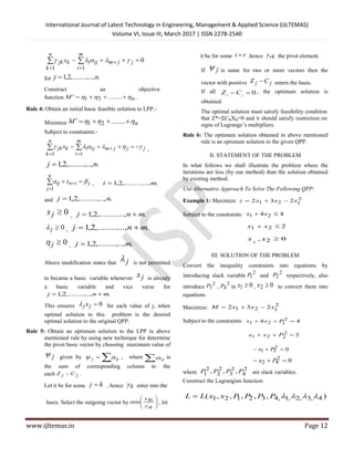
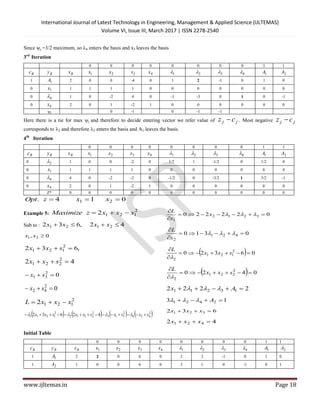
0 3x 6 2 3 1 0 0 0 0 0 0 0
0 4x 4 2 1 0 1 0 0 0 0 0 0
j 6 4 5 3
Since j =6 maximum, so x1 enters the basis and A1 leaves the basis.
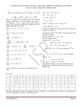
1st
Iteration
0 0 0 0 0 0 0 0 1 1
Bc By Bx 1x 2x 3x 4x 1 2 3 4 1A 2A
0 1x 1 1 0 0 0 1 1 -1/2 0 1/2 0
1 2A 1 0 0 0 0 3 1 0 -1 0 1
0 3x 4 0 3 1 0 -2 -2 1 0 -1/2 0
0 4x 2 0 1 0 1 -2 -2 1 0 -1/2 0
j 4 0 -2 3/2 -1 -1/2
Since j =4 maximum, so x2 enters the basis and x3 leaves the basis
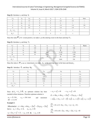
2nd
Iteration
0 0 0 0 0 0 0 0 1 1
Bc By Bx 1x 2x 3x 4x 1 2 3 4 1A 2A
0 1x 1 0 0 0 0 1 1 -1/2 0 0 1/2
1 2A 1 1 0 0 0 3 1 0 -1 1 0
0 2x 4/3 0 1 1/3 0 -2/4 -2/3 1/3 0 0 -1/4
0 4x 2/3 0 0 -1/3 1 -4/3 -4/3 2/3 0 0 -1/6
j 0 1/2 0 1/2 1/2
Since j =1/2 maximum, so 1 enters the basis and A2 leaves the basis
3rd
Iteration
0 0 0 0 0 0 0 0 1 1
Bc By Bx 1x 2x 3x 4x 1 2 3 4 1A 2A
0 1x 2/3 1 0 0 0 0 2/3 -1/2 1/3 1/2 -1/3
0 1 1/3 0 0 0 0 1 1/3 0 -1/3 0 1/3
0 2x 14/9 0 1 1/3 0 0 -4/9 1/3 -2/9 -1/6 2/3
0 4x 10/9 0 0 -1/3 1 0 -8/9 2/3 -4/9 -1/3 4/3
Z* 0 0 0 0 0 0 0 0 0 -1 -1
9
14
3
2
9
22
. 21  xxzOpt
.
IV. CONCLUSION
It is seen that the existing method is more inconvenient in
handling the degeneracy and cycling problems because here
the choice of the vectors, entering and outgoing, play an
important role. Here we observed that the optimum solution
obtained in three iterations by our modified technique, where
as Wolfe’s simplex method took five iterations. Hence our
technique gives efficiency in result as compared to other
method in less iteration. Hence the number of iterations
required is reduced by our methodology. Also we require less
time to simplify Numerical Problems.
REFERENCES
[1]. Wolfe P: “The Simplex method for Quadratic Programming”,
Econometrical, 27, 382-392., 1959.
[2]. Takayama T and Judge J. J : Spatial Equilibrium and
Quadratic Programming J. Farm Ecom.44, 67-93., 1964.
[3]. Terlaky T: A New Algorithm for Quadratic Programming
EJOOR, 32, 294- 301, North-Holland, 1984.
[4]. Ritter K : A dual Quadratic Programming Algorithm,
“University Of Wisconsin- Madison, Mathematics Research
Center. Technical Summary Report No.2733, 1952.
[5]. Frank M and Wolfe P: “An Algorithm for Quadratic
Programming”, Naval Research Logistic Quarterly, 3, 95-220.,
1956.
[6]. Khobragade N. W: Alternative Approach to Wolfe’s
Modified Simplex Method for Quadratic Programming
Problems, Int. J. Latest Trend Math, Vol.2 No. 1 March
2012. P. No. 1-18.

Optimum Solution of Quadratic Programming Problem: By Wolfe’s Modified Simplex Method

More Related Content

What's hot

Similar to Optimum Solution of Quadratic Programming Problem: By Wolfe’s Modified Simplex Method

More from IJLT EMAS

Recently uploaded

Optimum Solution of Quadratic Programming Problem: By Wolfe’s Modified Simplex Method