Lectures on Heat Transfer - Introduction - Applications - Fundamentals - Governing Laws

Lectures on Heat Transfer:
Introduction - Fundamentals
by
Dr. M. Thirumaleshwar
formerly:
Professor, Dept. of Mechanical Engineering,
St. Joseph Engg. College, Vamanjoor,
Mangalore

Preface
• This file contains Introduction to Heat
Transfer and Fundamental laws governing
heat transfer.
• The slides were prepared while teaching• The slides were prepared while teaching
Heat Transfer course to the M.Tech.
students in Mechanical Engineering Dept.
of St. Joseph Engineering College,
Vamanjoor, Mangalore, India, during Sept.
– Dec. 2010.
Aug. 2016 2MT/SJEC/M.Tech.

• It is hoped that these Slides will be useful
to teachers, students, researchers and
professionals working in this field.
• For students, it should be particularly
useful to study, quickly review the subject,useful to study, quickly review the subject,
and to prepare for the examinations.
•
Aug. 2016 3MT/SJEC/M.Tech.

References
• 1. Cengel Y. A. Heat Transfer: A Practical
Approach, 2nd Ed. McGraw Hill Co., 2003
• 2.Cengel, Y. A. and Ghajar, A. J., Heat and
Mass Transfer - Fundamentals and Applications,
5th Ed., McGraw-Hill, New York, NY, 2014.
Aug. 2016 MT/SJEC/M.Tech. 4
5th Ed., McGraw-Hill, New York, NY, 2014.
• 3. Incropera , Dewitt, Bergman, Lavine:
Fundamentals of Heat and Mass Transfer, 6th
Ed., Wiley Intl.
• 4. Necati Ozisik: Heat Transfer – A Basic
Approach, McGraw Hill

References… contd.
• 5. M. Thirumaleshwar: Fundamentals of Heat &
Mass Transfer, Pearson Edu., 2006
• 6. M. Thirumaleshwar: Software Solutions to
Problems on Heat Transfer – CONDUCTION-Problems on Heat Transfer – CONDUCTION-
Part-I, Bookboon, 2013
• http://bookboon.com/en/software-solutions-to-problems-on-
heat-transfer-ebook

Heat Transfer
Introduction - Fundamentals
• Applications - Modes of heat transfer-
Fundamental laws – governing rate
equations – concept of thermal resistance
equations – concept of thermal resistance
– general heat conduction equation –
different boundary conditions.

Applications of Heat Transfer:
• Mechanical Engineering: Boilers, Heat
Exchangers, Turbine systems, Internal
combustion engines etc.
• Metallurgical Engineering: Furnaces,
• Metallurgical Engineering: Furnaces,
Heat treatment of components etc.
• Electrical Engineering: Cooling systems
for electric motors, generators,
transformers etc.

Applications of Heat Transfer(Contd.)..
• Chemical Engineering: Process equipments
used in Refineries, Chemical plants etc.
• Nuclear Engineering: In removal of heat
generated by nuclear fission using liquid metal
generated by nuclear fission using liquid metal
coolants, design of nuclear fuel rods against
possible burn – out etc.
• Aerospace Engineering & Space Technology:
In the design of aircraft systems and
components, Rockets, Missiles etc.

Applications of Heat Transfer(Contd.)..
• Cryogenic Engineering: In the production,
storage, transportation and utilization of
cryogenic liquids (at very low temperatures
ranging from 100 K to 4 K or even lower) for
various Industrial, Research and Defence
applications.
applications.
• Civil Engineering: In the design of Suspension
bridges, railway tracks, Airconditioning and
Insulation of buildings etc.
• Principles and methods of Heat Transfer are
widely applied in many, many areas that affect
our lives.

Fundamental Laws governing
Heat Transfer:
– 1. First Law of Thermodynamics – gives
conservation of energy.
– 2. Second Law of Thermodynamics – gives
direction of heat flow.
direction of heat flow.
– 3. Equation of continuity – gives
conservation of mass.
– 4. Equation of flow – Newton’s Second Law
of motion—Navier Stokes’ Equations

Fundamental Laws governing
Heat Transfer (contd.):
– 5. Rate equations governing the three
modes of Heat Transfer:
– Conduction – Fourier’s Law of Conduction
– Convection – Newton’s Law of cooling
– Convection – Newton’s Law of cooling
– Radiation – Stefan – Boltzmann’s Law
– 6. Empirical relations for fluid properties
such as specific heat, thermal conductivity,
viscosity etc.
– 7. Equation of State for the fluid.

Modes of Heat Transfer
• Three main modes:
• Conduction …. heat flow by direct contact
• Convection … heat carried by moving fluid
• Radiation … heat flow does not need an• Radiation … heat flow does not need an
intervening medium
• In practical cases, a combination of one or
more of the above modes are present

Conduction:
• Governing ‘rate
equation’ for conduction
is: Fourier’s Law.
• Q = -k A (T2 – T1)/L
k
T1
Q
Slope = dT/dx
• Qx = -k A (T2 – T1)/L
...For a plane slab, in steady state
= k A (T1 – T2)/L
(Watts)
T2
X
L

Assumptions behind Fourier’s
Law:
• Fourier’s Law is an empirical law,
derived from experimental
observations and not from
fundamental, theoretical
considerations.
• Fourier’s Law is defined for steady
• Fourier’s Law is defined for steady
state, one dimensional heat flow.
• It is assumed that the bounding
surfaces between which heat flows
are isothermal and that the
temperature gradient is constant
i.e. the temperature profile is linear.

Assumptions behind Fourier’s
Law (contd.):
• There is no internal heat generation in the
material.
• The material is homogeneous (i.e. constant
density) and isotropic (i.e. thermal conductivity
density) and isotropic (i.e. thermal conductivity
is the same in all directions).
• Fourier’s Law is applicable to all states of
matter i.e. solid, liquid or gas.
• Fourier’s Law helps to define ‘thermal
conductivity’

Rate of heat transfer by conduction, Q, is given by:
L
T1
T2
Rate of heat transfer by conduction, Q, is given by:
Q = k A T/L (W)
where, k = thermal cond. (W/m.K)
A = Area of cross-section, (m^2)
L = Length, (m), T= temp. difference, (K)

Range of ‘k’ of various materials
at room temperature

Variation of ‘k’ with temperature

Variation of ‘k’ with temperature
for Cu and Al

Convection
• In convection, heat is
carried from place to
place by bulk movement
of fluidof fluid
• Convection currents are
set up when a pan of
water is heated

Newton’s Law of Cooling:
Q = h.A. T

Radiation
• energy is transferred by means of
electromagnetic waves.
• can take place through vacuum.
• can take place through vacuum.
• electromagnetic waves can propagate
through empty space.

Radiation
average frequency ∝ absolute temperature

Radiation

Greenhouse
Effect
Incoming UV radiation
from Sun easily passes
through the glass walls
of a greenhouse. Weaker
IR radiation, however,
IR radiation, however,
has difficulty passing
through the glass walls
and is trapped inside,
thus warming the
greenhouse.

Black body
A good absorber like
lampblack is also a
good emitter
good emitter
And, a poor
absorber like
polished silver is
also a poor emitter

The Stefan–Boltzmann Law
of Radiation
Rate of radiant energy emission is proportional to the
fourth power of its Absolute temperature.
Stefan’s law and is expressed as follows:
P = . . A. T4 (W)
P = . . A. T4 (W)
is the Stefan-Boltzmann constant, = 5.67 × 10-8 W/m2.K4.
is the emissivity, which is a number between 0 and 1.
T is the temp. in Kelvin

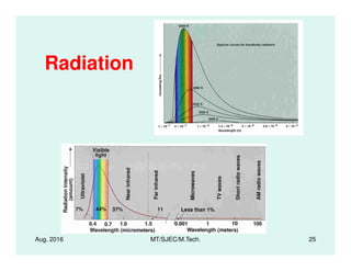
Radiation Heat Transfer
between bodies
• If the surrounding is at TS then the net
power radiated is:
P = A [ T4 - TS
4]
• Assuming on a dark, dry, night, T = 3 K:
• Assuming on a dark, dry, night, TS = 3 K:
• Frost may form even if air temperature >
0 C since radiation cools the surface
faster than conduction heat lost from the
ground or air.

Concept of Thermal resistance:
• Conduction:
• Q = kA(T1 – T2)/L
k
T1
T2
T(x)
Q
T2
X
L
Q
T1 T2
Rcond = L/kA
Q
Rth = L/(kA) is known as “Thermal resistance” of the slab for conduction.

Concept of Thermal resistance
(contd.):
• It is seen that there is a clear analogy between the flow
of heat and flow of electricity, as shown below:

(contd.):
• Convection heat transfer – thermal
resistance : U, Tf, h
Ts
Q
Q = h A (Ts – Tf)
Q Q
Ts Tf
Rconv = 1/hA
Rconv = 1/(hA)
Note that the Units are : (C/W) or (K/W)

(contd.):
• Radiation heat transfer – thermal resistance :
• Q1 = F1 A1 σ (T1
4 – T2
4), W
• F1 is known as view factor, which includes the effects of orientation,
emissivities and the distance between the surfaces

Practical applications of Thermal
resistance concept:
• To analyse the problems where one or
more modes of heat transfer occur
simultaneously
• To analyse the problems where multiple
• To analyse the problems where multiple
layers of materials of different thermal
conductivities are used; ex: in furnace
walls

Limitations for the use of
thermal resistance concept:
• Thermal concept can be used only
when all the following conditions are
satisfied:
• One dimensional conduction
• Steady state conduction
• No internal heat generation

Thermal diffusivity (αααα):
• Often, while dealing with transient
conduction problems, we come across a
quantity called ‘Thermal diffusivity’. Note
that Unit of α is: m2/s
that Unit of α is: m /s
Values of αααα for materials vary over a wide range:
For copper at room temperature, its value is approx. 113 * 10-6 m2/s
For glass it is about 0.34 * 10-6 m2/s.

Thermal diffusivity (αααα) for a few
materials at room temperature:

Thermal diffusivity (αααα) for a few materials
at room temperature(contd.):

GENERAL DIFFERENTIAL EQUATION
FOR HEAT CONDUCTION
• This is also known as ‘heat diffusion equation’ or,
simply ‘heat equation’.
• Consider a differential volume element (dx.dy.dz);
• Making an energy balance on this differential element:
Q
E
B
C
D
A
H
G
F
dx
dy
dzy
z
x
Qx Qx+dx
Qy
Qy+dy
Qz+dz
Qz

FOR HEAT CONDUCTION (contd.)
B
C
G
Fz
Qy+dy
Qz+dz
• Ein – Eout + Egen = Est …eqn. (1)
Energy, In
E
D
A
H
dx
dy
dzy
x
Qx Qx+dx
Qy
Qz
Energy, In
Energy, out
Energy, generated
Energy stored

Applying eqn (1):
where qg is the heat gen. rate per unit volume, (W/m3)
Now, etc.
eqn. (2)

Then, from eqn. (2):
But, from Fourier’s Law:
eqn. (3)
But, from Fourier’s Law:

Then, subst. in eqn. (3) and dividing by dx.dy.dz, we get:
eqn. (4)
This is the general form of heat diffusion
equation in Cartesian coordinates, for time
dependent (i.e. unsteady state) heat conduction,
with variable thermal conductivity and uniform heat
generation within the body.

Now, if the material is isotropic i.e. the thermal conductivity is
the same in all the three directions, i.e. kx = ky = kz = k say, :
eqn. (5)
If k is constant and does not vary with temperature
i.e. k does not change with position, then:
eqn. (6)

i.e.
eqn. (7)
where α = k/(ρcp) is thermal diffusivity, and
where α = k/(ρcp) is thermal diffusivity, and
∇ = Laplacian operator
Special cases:
1. Steady state: i.e.

eqn. (8)
Then, eqn. (7) becomes:
This is known as ‘Poisson equation’.
2. With no internal heat generation, i.e. qg = 0:
Then, eqn. (7) becomes:
eqn. (9)
This is known as ‘Diffusion equation’.

3. Steady state, with no internal heat generation, i.e.
eqn. (10)
τ∂
∂T
Therefore,
This is known as ‘Laplace equation’.
4. One dimensional, steady state, with no internal heat generation,
i.e.
Therefore,

eqn. (11)
So, equation (7) becomes:

in cylindrical coordinates:
eqn. (12)
For one dimensional conduction in r - direction only, we get:
eqn. (13)

in spherical coordinates:
eqn. (14)
For one dimensional conduction in r - direction only, we
get:
eqn. (15)

Boundary and Initial conditions:
Commonly encountered Boundary Conditions (B.C’s) are:
• Prescribed temperature conditions at the
boundaries – known as B.C. of the first
kind or Dirichlet condition:

• Prescribed heat flux condition at the
boundaries - known as B.C. of the
second kind or Neumann condition

Prescribed heat flux condition at the
boundaries:
Two special cases:
1. Insulated boundary: 2. Thermal symmetry:

• Convection boundary condition - known
as B.C. of the third kind:

• Interface boundary condition - known as
B.C. of the fourth kind:

• Example3.1: Temperature variation in a slab is
given by: T(x) = 100 + 200 x –500 x2, where x is in
metres; x = 0 at the left face and x = 0.3 m at the
right face. Thermal conductivity of the material k =
45 W/(m.C). Also, cp = 4 kJ/(kg.K) and ρρρρ = 1600
kg/m3. Determine:
• Temperature at both surfaces
• Heat transfer at left face and its direction
• Heat transfer at right face and its direction
• Heat transfer at right face and its direction
• Is there any heat generation in the slab? If so, how
much?
• Max. temperature in the slab and its location
• Time rate of change of temperature at x = 0.1 m if
the heat generation rate is suddenly doubled
• Draw the temperature profile in the slab

k, qg
Temp. Profile
QrightQleft
Data:
L 0.3 m
k 45 W/m.C
c p 4000 J/kg.K
ρ 1600 kg/m^3
α
k
L
α
k
ρ c p
.
α 7.031 10
6
= m2/s
Fig. Ex. 3.1 (a)

T x( ) 100 200 x. 500 x
2. Define T(x)...i.e. temp. as a function of x
Temp. at left face: i.e. at x = 0: T 0( ) 100= C....Ans.
Temp. at right face: i.e. at x = 0.3 m: T 0.3( ) 115= C....Ans.
To find max. temp.:
Define the first derivative of T(x): T' x( )
x
T x( )
d
d
Also, define the second derivative of T(x): T'' x( )
x
T' x( )
d
d
--------------------------------------------------------------------------------------------------------------------------

• By hand calculation:
• We get: T`(x) = 200 –1000.x
• We set T`(x) equal to zero to get the
position xmax where temp. is max.:
• i.e. 200 – 1000.x = 0.
• This gives x = 0.2 m. Substitute this value
• This gives x = 0.2 m. Substitute this value
of xmax in T(x) to get the value of Tmax.
• So, Tmax = T(0.2) =
100 + 200 x 0.2 – 500 x (0.2)2. = 120 C.

Temp. distribution in the slab:
T x( )
110
115
120
Variation of T(x) with x for Slab
x
0 0.1 0.2 0.3
100
105
Fig. Ex. 3.1 (b)
Note from the graph that the max. temp. occurs at x = 0.2 m and its value is 120 C, as
already calculated.

To calculate the heat fluxes at the left and right faces :
Apply the Fourier's Law at x = 0 and at x = 0.3 m, remembering that temp. gradient is
given by T'(x), aready defined.
q left k T' 0( ). ..applying Fourier's Law at left face i.e. at x = 0
q left 9 10
3
= ...Heat flux at the left face (W/m^2) ; note that -ve sign indicates
heat flowing from right to left
q right k T' 0.3( ). ..applying Fourier's Law at right face i.e. at x = 0
q right 4.5 10
3
= ...Heat flux at the right face (W/m^2 ); note that +ve sign indicates
heat flowing from left to right.
q total q left q right ...Total heat generated per m^2 of surface
q total 1.35 10
4
= W/m^2...Total heat generated/m^2

• To calculate the time rate of change of temperature
at x = 0.1 m when qg is suddenly doubled:
• We have the time dependent differential equation for
Therefore, qg, the volumetric heat gen. rate is given by Total heat gen. per unit volume:
q g
q total
1 0.3.
q g 4.5 10
4
= W/m^3...vol. heat gen. rate in the slab....Ans .
• We have the time dependent differential equation for
heat conduction in Cartesian coordinates:
τατ
ρ
∂
∂
=
∂
∂
=+
∂
∂ TT
k
c
k
q
x
T pg 1
2
2

• Therefore,
αα
τ k
q
x
TT g
+
∂
∂
=
∂
∂
2
2
From the given equation for temperature distribution,
it is clear that does not depend on x, i.e.
depends only on qg:
2
2
x
T
∂
∂
τ∂
∂T
depends only on qg:
τ∂
dtbyd τ x( ) α T'' x( ). α
2 q g
.
k
. ...define dT/d ττττ as a function x . Now, we can get dT/dτ
at any x by simply substituting that value of x in the
function defined
dtbyd τ 0.1( ) 7.031 10
3
= C/s....time rate of change of temp. ...Ans.
Note that this is true for all x since T''(x) does not depend on x
for the temperature distribution given

• Example 1.3 : Electronic power devices
are mounted to a heat sink having an
exposed surface area of 0.045 m^2 and
an emissivity of 0.8. When the devices
dissipate a total power of 20 W and air
and surroundings are at 27 C, theand surroundings are at 27 C, the
average sink temperature is 42 C. What
average temperature will the heat sink
reach when the devices dissipate 30 W
for the same environmental
conditions?

Variation of T2 with epsilon:

Lectures on Heat Transfer - Introduction - Applications - Fundamentals - Governing Laws

More Related Content

What's hot

Viewers also liked

Similar to Lectures on Heat Transfer - Introduction - Applications - Fundamentals - Governing Laws

More from tmuliya

Recently uploaded

Lectures on Heat Transfer - Introduction - Applications - Fundamentals - Governing Laws